Generate Traversability Map for Offroad Terrain Using Semantic Segmentation

Since R2026a

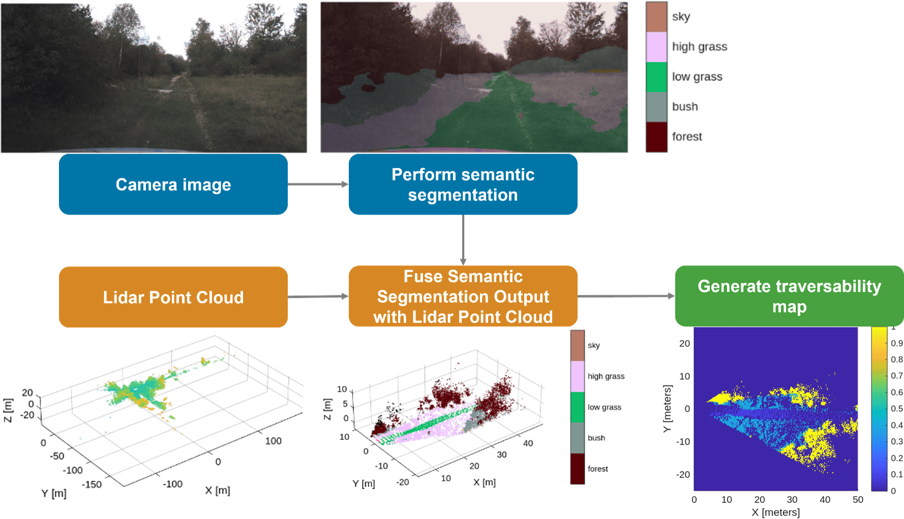
This example shows how to create a real-time traversability map for an offroad terrain by fusing semantic segmentation from camera images with lidar point clouds. The map assigns costs to terrain regions based on navigability, enabling safe and efficient path planning for autonomous vehicles.

The workflow uses the German Outdoor and Offroad Dataset (GOOSE) [1] data set, which provides synchronized camera and lidar data for offroad driving scenarios. The process is organized into the following steps:

• Load and Visualize Offroad Sensor Data

• Perform 2-D Semantic Segmentation On Camera Image

• Fuse Semantic Segmentation Output With Lidar Point Cloud

• Generate Traversability Map From Semantic Point Cloud

• Update Traversability Map in Loop for Driving Sequence

Prerequisites

This example uses the Offroad Autonomy for Heavy Machinery to create the traversabilityMap object. Additionally, you also need these toolboxes:

• ROS Toolbox™— Open and parse driving data ROS bag file using rosbag (ROS Toolbox) function, extract image and point cloud using rosReadImage (ROS Toolbox),rosReadXYZ (ROS Toolbox) functions.

• Deep Learning Toolbox Converter for PyTorch Models— Import pretrained deep learning model using importNetworkFromPyTorch (Deep Learning Toolbox) to perform 2-D semantic segmentation on camera images.

• Deep Learning Toolbox™ — Store pretrained model using the dlnetwork (Deep Learning Toolbox) object and extract network predictions using the predict (Deep Learning Toolbox) function.

• Computer Vision Toolbox™ — Convert camera intrinsic parameters from OpenCV to MATLAB using cameraIntrinsicsFromOpenCV (Computer Vision Toolbox) and perform camera to lidar coordinate transformation using rigidtform3d (Image Processing Toolbox).

• Lidar Toolbox™— Fuse image to lidar point cloud using fuseCameraToLidar function and perform point cloud processing with functions such as findPointsInROI (Computer Vision Toolbox), and select (Computer Vision Toolbox).

Load and Visualize Offroad Sensor Data

Download the offroad driving data stored in a ROS bag file named drivingScenarioGOOSE.bag (1 GB in size). This data set is part of the GOOSE data set [1]. It contains the images from the windshield-mounted RGB camera and 3-D point clouds from a roof-mounted lidar sensor. For more details about how the data was extracted, refer to drivingScenarioGOOSE.txt, which is included with the ROS bag file.

drivingDataRosbagFile = "drivingScenarioGOOSE.bag";
if ~exist(drivingDataRosbagFile, "file")
    filename = matlab.internal.examples.downloadSupportFile("robotics/data", "drivingScenarioGOOSE.zip");
    unzip(filename)
end

You can visualize the contents of the rosbag file using the ROS Data Analyzer (ROS Toolbox) app. You can observe and correlate features such as trees and bushes between the camera images and the lidar point clouds.

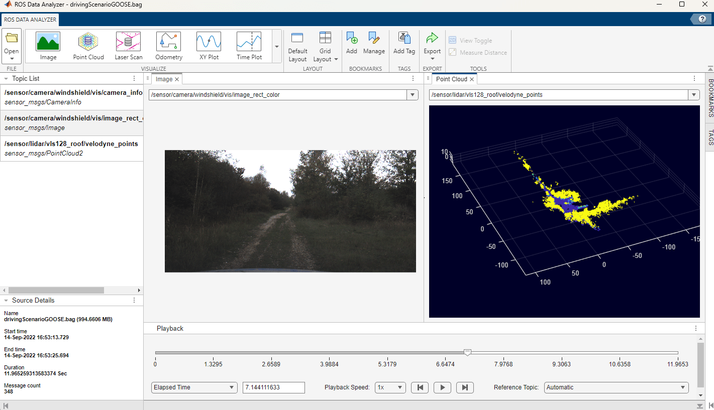
Open and parse the driving data rosbag file. In this example, you extract camera images, camera info, and lidar point clouds from this file.

drivingDataRosbag = rosbag(drivingDataRosbagFile);

Open and parse the ROS bag file named staticTransformsMuCAR-3.bag. This file contains coordinate frames of various vehicle sensors and their relationships in a tree structure. In this example, you extract the camera-to-lidar coordinate transformation matrix from the file.

tfTreeRosbag = rosbag("staticTransformsMuCAR-3.bag");

The helper function helperReadRosbagData helps you to extract the data from the ros bag objects, including the synchronized camera images and lidar point clouds. Additionally, it imports parameters related to camera intrinsics, camera region of interest, and camera-to-lidar transform. This helper function utilizes ROS Toolbox™ functions such as rosReadImage (ROS Toolbox),and rosReadXYZ (ROS Toolbox) to convert the camera images and 3-D point clouds from ROS messages into MATLAB. It also utilizes Computer Vision Toolbox™ functions such as cameraIntrinsicsFromOpenCV (Computer Vision Toolbox) to import camera parameters from OpenCV to MATLAB, and rigidtform3d (Image Processing Toolbox) to store the camera-to-lidar coordinate transformation.

[cameraImages, lidarPointClouds, cameraIntrinsicParams, cameraROIParams, cameraToLidarTf] ...
    = helperReadRosbagData(DrivingDataRosbag=drivingDataRosbag, TfTreeRosBag=tfTreeRosbag);

Perform 2-D Semantic Segmentation on Camera Image

Download the pretrained semantic segmentation model file named ppliteSegClass512GOOSE.pt (50MB in size). This PyTorch model was trained on the GOOSE data set [1] and is based on PP‑LiteSeg [2], which employs a lightweight neural network architecture and is capable of real-time performance.

pytorchModel = "ppliteSegClass512GOOSE.pt";
if ~exist(pytorchModel, "file")
    filename = matlab.internal.examples.downloadSupportFile("robotics/data", "ppliteSegClass512GOOSE.zip");
    unzip(filename)
end

Import the PyTorch model into MATLAB using importNetworkFromPyTorch from Deep Learning Toolbox Converter for PyTorch Models. The software displays a standard warning with information on adding the input layer and initializing the network.

net = importNetworkFromPyTorch(pytorchModel);

Importing the model, this may take a few minutes...

Warning: Some issues were found during translation, but no placeholders were generated:
Trained variances in BatchNormalization layer 'aten::batch_norm' must be nonnegative. Zero or negative values were imported as small positive values.

Warning: Network was imported as an uninitialized dlnetwork. Before using the network, add input layers:

% Create imageInputLayer for the network input at index 1:
inputLayer1 = imageInputLayer(<inputSize1>, Normalization="none");

% Add input layers to the network and initialize:
net = addInputLayer(net, inputLayer1, Initialize=true);

Define the input layer size to match the image dimensions used for training the PyTorch model. The original camera images of size [1024 × 2048] pixels were resized to enable faster training while preserving high accuracy. During inference, the camera images are resized at the network input to match the expected input layer size.

inputLayerSize = [768, 768, 3];

Use inputLayerSize for creating the input layer. Add the input layer and initialize the network as described in the standard warning above.

inputLayer = imageInputLayer(inputLayerSize, Name="imageinput_1", Normalization="none");
net = addInputLayer(net, inputLayer, Initialize=true);

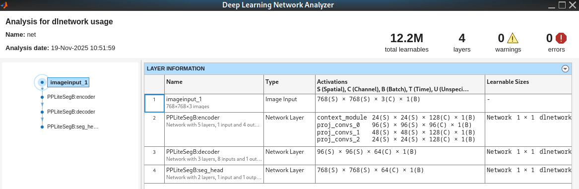
You can visualize the imported network using the analyzeNetwork (Deep Learning Toolbox) app by running the command analyzeNetwork(net). The first layer is an image input layer. The second and third layers contain the encoder-decoder architecture. The last layer is the semantic segmentation head, which outputs the probabilities of 64 offroad object classes for each pixel in the input image, as defined by the GOOSE data set labeling policy [3].

Load a camera image.

frameIdx = 1;
cameraImage = cameraImages{frameIdx};

The helper function, helperSegmentCameraImage, segments the camera image with the pretrained network, net. The function predicts the semanticID for each pixel in the image.

semanticID = helperSegmentCameraImage(net, cameraImage);

The semanticID output predicts one of 64 object types. The GOOSE labeling policy assigns each semantic class a unique ID and a specific RGB color value. This image illustrates these assignments for the objects identified in the off-road driving scenario used in this example.

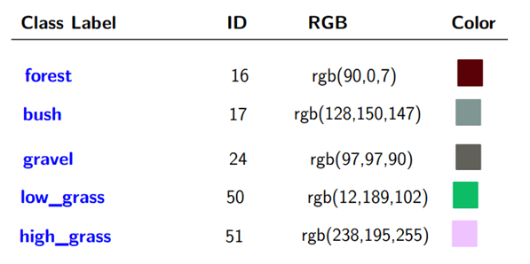
Load the semantic information for the 64 classes defined in the GOOSE data set [3]. The ClassToId provides the mapping between class label and semanticID. The ClassToRGB field provides the mapping between class label and the RGB color.

Load the GOOSE data set semantic information using the SemanticClassInfo class. The ClassToId property maps each class label to its semanticID, and the ClassToRGB property maps each class label to its RGB color value.

semanticInfo = SemanticClassInfo

semanticInfo = 
  SemanticClassInfo with properties:

     ClassToID: dictionary (string ⟼ double) with 64 entries
    ClassToRGB: dictionary (string ⟼ cell) with 64 entries

Extract the semantic image, semanticImage, from the semanticID. This image contains the RGB colors representing the semantic segmentation. Fuse semanticImage with the 3-D point cloud to create a semantic point cloud, which you will use later to construct a traversability map.

semanticImage = helperSemanticImageFromID(semanticID, SemanticInfo=semanticInfo);

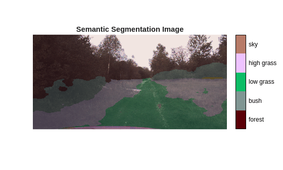
Display semantic image overlaid on the camera image along with a legend showing the class names.

figure
colormapData = double(cell2mat(semanticInfo.ClassToRGB.values))/255.;
semanticOverlayImage = labeloverlay(cameraImage, semanticID, ColorMap=colormapData, Transparency=0.8);
imshow(semanticOverlayImage, InitialMagnification='fit')
helperShowSemanticLegend(semanticID, SemanticInfo=semanticInfo);
title('Semantic Segmentation Image')

Fuse Semantic Image with Lidar Point Cloud

Load the point cloud corresponding to the camera frame used in the previous section.

ptCloud = pointCloud(lidarPointClouds{frameIdx});

The original camera images have been cropped at the top based on the region of interest parameters, cameraROIParams. Pad the semantic image at the top to align with original image coordinate system.

yoffset = double(cameraROIParams.YOffset);
paddedSemanticRGB = padarray(semanticImage, [yoffset, 0], 0, 'pre');

Fuse the semantic image with the lidar point cloud using the camera's intrinsic parameters and the camera-to-lidar coordinate transformation matrix.

[semanticPtCloud, ~, ptCloudIdx] = fuseCameraToLidar(paddedSemanticRGB, ptCloud,...
    cameraIntrinsicParams, cameraToLidarTf);

Select only the fused point cloud points in the camera field of view.

semanticPtCloud = select(semanticPtCloud, ptCloudIdx);

Define the xy limits to include only the region of interest around the vehicle for traversability map estimation. For motion planning, use points ahead of the vehicle, as well as the points to the left and right sides of the vehicle.

mapLimits = [0, 50;   % x-limits include points up to 50 meters in front of the lidar sensor
           -25, 25];  % y-limits include points up to 25 meters to the left & right of the lidar sensor           
pointCloudROI = [mapLimits; semanticPtCloud.ZLimits];

idx = findPointsInROI(semanticPtCloud, pointCloudROI);
semanticPtCloud = select(semanticPtCloud, idx);

Display the semantically labeled point cloud for selected region of interest. Also display the legend that links the semantic RGB colors to the class names.

figure
pcshow(semanticPtCloud, Background="w")
hold on
helperShowSemanticLegend(semanticID, SemanticInfo=semanticInfo);
xlabel('X [m]')
ylabel('Y [m]')
zlabel('Z [m]')
title('Semantic Point Cloud')

Generate Traversability Map from Semantic Point Cloud

Define the traversability map dimensions, resolution, and grid origin based on the spatial bounds used in the previous section.

mapWidth = mapLimits(1,2)-mapLimits(1,1);  % meters
mapHeight = mapLimits(2,2)-mapLimits(2,1); % meters
gridOriginInLocal = [mapLimits(1,1), mapLimits(2,1)]; % Location of the bottom-left corner of the map grid in local coordinates
mapResolution = 5; % cells per meter

Create an empty traversabilityMap object. This map is updated in real-time based on the most recent semantic point cloud data captured from the camera and lidar sensors.

map = traversabilityMap(mapWidth, mapHeight, mapResolution);
map.GridOriginInLocal = gridOriginInLocal;

Define traversability costs for different semantic classes. Add a new field ClassToCost to semanticInfo to store the semantic cost information for various classes. By default, assign a cost of 1.0 (non-traversable) to classes such as "forest", "bush", and "unknown". For classes such as "low grass", "bush", "gravel", define costs in the range 0.0 ≤ cost ≤ 1.0, where a lower cost indicates higher traversability.

semanticInfo.ClassToCost("asphalt") = 0.0;
semanticInfo.ClassToCost("low grass") = 0.1;
semanticInfo.ClassToCost("soil") = 0.2;
semanticInfo.ClassToCost("high grass") = 0.4;
semanticInfo.ClassToCost("gravel") = 0.5;
semanticInfo.ClassToCost("cobble") = 0.7;

Convert the semantically segmented 3-D point cloud into a 2-D grid representation. For each grid cell, the function assigns a semantic cost based on the most frequently occurring class below a height threshold. It filters out objects above this threshold that do not affect terrain traversability, such as "sky", and "tree crown".

[semanticCost,...    % Semantic costs for grid cells where available (N x 1 array)
    gridLocation]... % [row, col] indices of grid cells for which semantic cost is available (N x 2 array)
    = helperSemanticPointCloudToGrid(semanticPtCloud,...
        GridSize=map.GridSize, XYLimits=mapLimits, SemanticInfo=semanticInfo);

Set the traversability map using the semantic cost data for grid locations where it is available.

setMapData(map, 'Semantic', gridLocation, semanticCost, "grid");

Show the updated traversability map. Regions with lower costs (closer to 0.0) have higher traversability, and regions with higher costs (closer to 1.0) have lower traversability.

figure
show(map)
title("Traversability map")

You can also query cost at any given location using the cost method of the traversabilityMap object. For example, you can query the cost at a specific xy location as shown in this code:

xy = [20, -5; 40, -15];
cost(map, xy)

ans = 2×1

         0
    0.7000

Update Traversability Map in Loop for Driving Sequence

In real-world autonomous driving, the map is continuously updated in real time using the latest sensor data. You can simulate this by combining the previously discussed steps and executing them iteratively for each timestamp in the driving sequence.

% Create empty traversability map
mapResolution = 2.5; % lower resolution => faster simulation, but lower accuracy
map = traversabilityMap(mapWidth, mapHeight, mapResolution,...
    GridOriginInLocal = gridOriginInLocal);

% Flag to indicate whether the plot has been initialized; set to true once
% the axes object is created for reuse in subsequent iterations
isPlotInit = false;

% Higher frame skip interval => faster simulation
frameSkipInterval = 2;

% Rate control at 1Hz
rateObj = rateControl(1);

for i = 1:frameSkipInterval:length(cameraImages)

    %-----------------------------------------
    % Step 1: Read Imported Offroad Driving Data from Pre-recorded Rosbag
    %----------------------------------------
    cameraImage = cameraImages{i};
    ptCloud = pointCloud(lidarPointClouds{i});    

    %-----------------------------------------
    % Step 2: Perform 2D Semantic Segmentation on Camera Image
    %-----------------------------------------

    % Class label ID prediction from semantic segmentation
    semanticID = helperSegmentCameraImage(net, cameraImage);

    % Extract semantic RGB image from semantic ID prediction 
    [semanticImage] = helperSemanticImageFromID(semanticID, SemanticInfo=semanticInfo);

    %-----------------------------------------
    % Step 3: Fuse Semantic Image with Lidar Point Cloud
    %-----------------------------------------
    % Pad semantic image based on ROI in camera parameters
    yoffset = double(cameraROIParams.YOffset);
    semanticImage = padarray(semanticImage, [yoffset, 0], 0, 'pre'); 

    % Extract semantic point cloud by fusing semantic RGB image to the
    % point cloud
    ptCloud = pcdenoise(ptCloud);
    [semanticPtCloud, ~, ptCloudIdx] = fuseCameraToLidar(semanticImage, ptCloud,...
        cameraIntrinsicParams, cameraToLidarTf);
    semanticPtCloud = select(semanticPtCloud, ptCloudIdx);

    % Filter ROI in semantic point cloud
    pointCloudROI = [mapLimits; semanticPtCloud.ZLimits];
    ptCloudIdx = findPointsInROI(semanticPtCloud, pointCloudROI);
    semanticPtCloud = select(semanticPtCloud, ptCloudIdx);
    
    %-----------------------------------------
    % Step 4: Generate Traversability Map from Semantic Point Cloud
    %-----------------------------------------
    % Extract semantic cost from semantic point cloud
    [semanticCost, gridLocation] = helperSemanticPointCloudToGrid(semanticPtCloud,...        
        GridSize=map.GridSize, XYLimits=mapLimits, SemanticInfo=semanticInfo);

    % Update traversability map data
    setMapData(map, 'Semantic', gridLocation, semanticCost, "grid");
    

    %-----------------------------------------
    %Step 5: Visualize semantic segmentation and traversability map
    %-----------------------------------------
    if ~isPlotInit  
        figure('Position', [100, 100, 800, 600]);
        axesobj = helperShowSemanticTraversability(CameraImage=cameraImage, SemanticID=semanticID,...
            SemanticInfo=semanticInfo, Map=map);
        isPlotInit = true;        
    else
        helperShowSemanticTraversability(CameraImage=cameraImage, SemanticID=semanticID,...
            SemanticInfo=semanticInfo, Map=map, AxesObj=axesobj);
    end

    waitfor(rateObj);
end

Conclusion

This example shows how to generate a real-time local traversability cost map for an offroad terrain by fusing semantic segmentation from camera images with lidar point cloud data. The resulting traversability map can then be used to plan the vehicle motion in real-time. The traversability map assigns costs to different regions based on their navigability, where lower costs indicate easily traversability terrain such as roads, and higher costs represent obstacles or challenging terrain such as bushes and trees. You can use the resulting traversability cost map to plan safe and efficient paths for the vehicle using motion planning algorithms such as plannerHybridAStar (Navigation Toolbox), offroadControllerMPPI.

References

[1] Mortimer, Peter, Raphael Hagmanns, Miguel Granero, Thorsten Luettel, Janko Petereit, and Hans-Joachim Wuensche. “The GOOSE Dataset for Perception in Unstructured Environments.” Proceedings of IEEE International Conference on Robotics and Automation (ICRA), 2024. https://arxiv.org/abs/2310.16788.

[2] Zhao, Zilong, Xuecheng Wang, Yifan Sun, and Shumin Han. "PP-LiteSeg: A Superior Real-Time Semantic Segmentation Model." Proceedings of the IEEE/CVF Conference on Computer Vision and Pattern Recognition (CVPR), 2022. https://arxiv.org/abs/2204.02681

[3] Mortimer, Peter, and Juan David González. "GOOSE Dataset Labeling Policy: Class Definitions and Examples for the Labeling Process." Universität der Bundeswehr München, Fakultät für Luft- und Raumfahrttechnik, Institut für Technik Autonomer Systeme, UniBwM / LRT / TAS / TR 2022:1, 20 October 2023. https://goose-dataset.de/docs/resources/labeling_policy.pdf

[4] Guan, Tianrui, Zhenpeng He, Dinesh Manocha, and Liangjun Zhang. "TTM: Terrain Traversability Mapping for Autonomous Excavator Navigation in Unstructured Environments." arXiv preprint arXiv:2109.06250, 2022. https://arxiv.org/abs/2109.06250.