Contenuto principale
Risultati per
This is Stella while waiting to see if the code works...

I'm excited to share some valuable resources that I've found to be incredibly helpful for anyone looking to enhance their MATLAB skills. Whether you're just starting out, studying as a student, or are a seasoned professional, these guides and books offer a wealth of information to aid in your learning journey.
These materials are freely available and can be a great addition to your learning resources. They cover a wide range of topics and are designed to help users at all levels to improve their proficiency in MATLAB.
Happy learning and I hope you find these resources as useful as I have!
I found this link posted on Reddit.
https://workhunty.com/job-blog/where-is-the-best-place-to-be-a-programmer/Matlab/

Let S be the closed surface composed of the hemisphere  and the base
  Let
Let  be the electric field defined by
  . Find the electric flux through S. (Hint: Divide S into two parts and calculate
  ).
).
% Define the limits of integration for the hemisphere S1
theta_lim = [-pi/2, pi/2];
phi_lim = [0, pi/2];
% Perform the double integration over the spherical surface of the hemisphere S1
% Define the electric flux function for the hemisphere S1
flux_function_S1 = @(theta, phi) 2 * sin(phi);
electric_flux_S1 = integral2(flux_function_S1, theta_lim(1), theta_lim(2), phi_lim(1), phi_lim(2));
% For the base of the hemisphere S2, the electric flux is 0 since the electric
% field has no z-component at the base
electric_flux_S2 = 0;
% Calculate the total electric flux through the closed surface S
total_electric_flux = electric_flux_S1 + electric_flux_S2;
% Display the flux calculations
disp(['Electric flux through the hemisphere S1: ', num2str(electric_flux_S1)]);
disp(['Electric flux through the base of the hemisphere S2: ', num2str(electric_flux_S2)]);
disp(['Total electric flux through the closed surface S: ', num2str(total_electric_flux)]);
% Parameters for the plot
radius = 1; % Radius of the hemisphere
% Create a meshgrid for theta and phi for the plot
[theta, phi] = meshgrid(linspace(theta_lim(1), theta_lim(2), 20), linspace(phi_lim(1), phi_lim(2), 20));
% Calculate Cartesian coordinates for the points on the hemisphere
x = radius * sin(phi) .* cos(theta);
y = radius * sin(phi) .* sin(theta);
z = radius * cos(phi);
% Define the electric field components
Ex = 2 * x;
Ey = 2 * y;
Ez = 2 * z;
% Plot the hemisphere
figure;
surf(x, y, z, 'FaceAlpha', 0.5, 'EdgeColor', 'none');
hold on;
% Plot the electric field vectors
quiver3(x, y, z, Ex, Ey, Ez, 'r');
% Plot the base of the hemisphere
[x_base, y_base] = meshgrid(linspace(-radius, radius, 20), linspace(-radius, radius, 20));
z_base = zeros(size(x_base));
surf(x_base, y_base, z_base, 'FaceColor', 'cyan', 'FaceAlpha', 0.3);
% Additional plot settings
colormap('cool');
axis equal;
grid on;
xlabel('X');
ylabel('Y');
zlabel('Z');
title('Hemisphere and Electric Field');

Although, I think I will only get to see a partial eclipse (April 8th!) from where I am at in the U.S. I will always have MATLAB to make my own solar eclipse. Just as good as the real thing.
Code (found on the @MATLAB instagram)
a=716;
v=255;
X=linspace(-10,10,a);
[~,r]=cart2pol(X,X');
colormap(gray.*[1 .78 .3]);
[t,g]=cart2pol(X+2.6,X'+1.4);
image(rescale(-1*(2*sin(t*10)+60*g.^.2),0,v))
hold on
h=exp(-(r-3)).*abs(ifft2(r.^-1.8.*cos(7*rand(a))));
h(r<3)=0;
image(v*ones(a),'AlphaData',rescale(h,0,1))
camva(3.8)

One of the privileges of working at MathWorks is that I get to hang out with some really amazing people. Steve Eddins, of ‘Steve on Image Processing’ fame is one of those people. He recently announced his retirement and before his final day, I got the chance to interview him. See what he had to say over at The MATLAB Blog The Steve Eddins Interview: 30 years of MathWorking
Before we begin, you will need to make sure you have 'sir_age_model.m' installed. Once you've downloaded this folder into your working directory, which can be located at your current folder. If you can see this file in your current folder, then it's safe to use it. If you choose to use MATLAB online or MATLAB Mobile, you may upload this to your MATLAB Drive.
This is the code for the SIR model stratified into 2 age groups (children and adults). For a detailed explanation of how to derive the force of infection by age group.
% Main script to run the SIR model simulation
% Initial state values
initial_state_values = [200000; 1; 0; 800000; 0; 0]; % [S1; I1; R1; S2; I2; R2]
% Parameters
parameters = [0.05; 7; 6; 1; 10; 1/5]; % [b; c_11; c_12; c_21; c_22; gamma]
% Time span for the simulation (3 months, with daily steps)
tspan = [0 90];
% Solve the ODE
[t, y] = ode45(@(t, y) sir_age_model(t, y, parameters), tspan, initial_state_values);
% Plotting the results
plot(t, y);
xlabel('Time (days)');
ylabel('Number of people');
legend('S1', 'I1', 'R1', 'S2', 'I2', 'R2');
title('SIR Model with Age Structure');

What was the cumulative incidence of infection during this epidemic? What proportion of those infections occurred in children?
In the SIR model, the cumulative incidence of infection is simply the decline in susceptibility.
% Assuming 'y' contains the simulation results from the ode45 function
% and 't' contains the time points
% Total cumulative incidence
total_cumulative_incidence = (y(1,1) - y(end,1)) + (y(1,4) - y(end,4));
fprintf('Total cumulative incidence: %f\n', total_cumulative_incidence);
% Cumulative incidence in children
cumulative_incidence_children = (y(1,1) - y(end,1));
% Proportion of infections in children
proportion_infections_children = cumulative_incidence_children / total_cumulative_incidence;
fprintf('Proportion of infections in children: %f\n', proportion_infections_children);
927,447 people became infected during this epidemic, 20.5% of which were children.
Which age group was most affected by the epidemic?
To answer this, we can calculate the proportion of children and adults that became infected.
% Assuming 'y' contains the simulation results from the ode45 function
% and 't' contains the time points
% Proportion of children that became infected
initial_children = 200000; % initial number of susceptible children
final_susceptible_children = y(end,1); % final number of susceptible children
proportion_infected_children = (initial_children - final_susceptible_children) / initial_children;
fprintf('Proportion of children that became infected: %f\n', proportion_infected_children);
% Proportion of adults that became infected
initial_adults = 800000; % initial number of susceptible adults
final_susceptible_adults = y(end,4); % final number of susceptible adults
proportion_infected_adults = (initial_adults - final_susceptible_adults) / initial_adults;
fprintf('Proportion of adults that became infected: %f\n', proportion_infected_adults);
Throughout this epidemic, 95% of all children and 92% of all adults were infected. Children were therefore slightly more affected in proportion to their population size, even though the majority of infections occurred in adults.
Are you going to be in the path of totality? How can you predict, track, and simulate the solar eclipse using MATLAB?
In one line of MATLAB code, compute how far you can see at the seashore. In otherwords, how far away is the horizon from your eyes? You can assume you know your height and the diameter or radius of the earth.
Keep calm and study PDEs

Me at the beginning of every meeting

A bit late. Compliments to Chris for sharing.
The latest release is pretty much upon us. Official annoucements will be coming soon and the eagle-eyed among you will have started to notice some things shifting around on the MathWorks website as we ready for this.
The pre-release has been available for a while. Maybe you've played with it? I have...I've even been quietly using it to write some of my latest blog posts...and I have several queued up for publication after MathWorks officially drops the release.
At the time of writing, this page points to the pre-release highlights. Prerelease Release Highlights - MATLAB & Simulink (mathworks.com)
What excites you about this release? why?
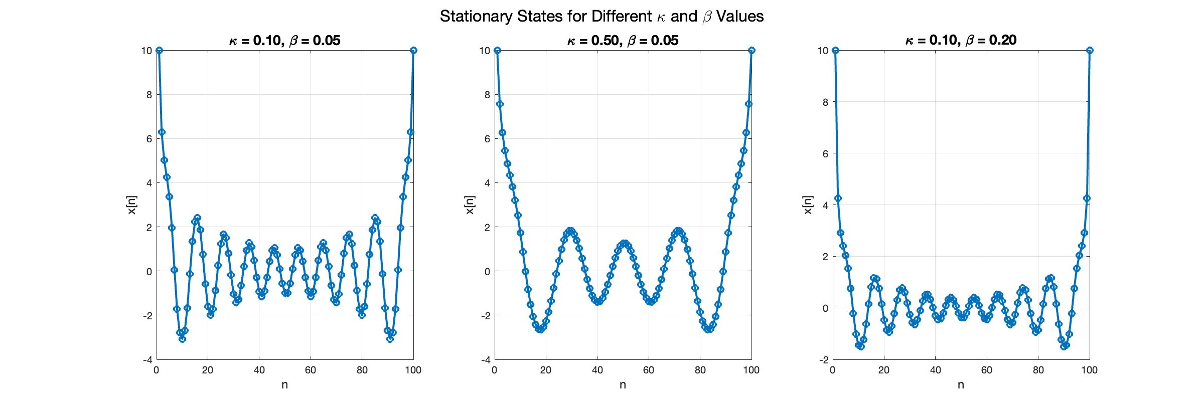
The stationary solutions of the Klein-Gordon equation refer to solutions that are time-independent, meaning they remain constant over time. For the non-linear Klein-Gordon equation you are discussing:

Stationary solutions arise when the time derivative term,  , is zero, meaning the motion of the system does not change over time. This leads to a static differential equation:
 , is zero, meaning the motion of the system does not change over time. This leads to a static differential equation:
This equation describes how particles in the lattice interact with each other and how non-linearity affects the steady state of the system.
The solutions to this equation correspond to the various possible stable equilibrium states of the system, where each represents different static distribution patterns of displacements  . The specific form of these stationary solutions depends on the system parameters, such as κ , ω, and β , as well as the initial and boundary conditions of the problem.
To find these solutions in a more specific form, one might need to solve the equation using analytical or numerical methods, considering the different cases that could arise in such a non-linear system.
By interpreting the equation in this way, we can relate the dynamics described by the discrete Klein - Gordon equation to the behavior of DNA molecules within a biological system . This analogy allows us to understand the behavior of DNA in terms of concepts from physics and mathematical modeling .
% Parameters
numBases = 100; % Number of spatial points
omegaD = 0.2; % Common parameter for the equation
% Preallocate the array for the function handles
equations = cell(numBases, 1);
% Initial guess for the solution
initialGuess = 0.01 * ones(numBases, 1);
% Parameter sets for kappa and beta
paramSets = [0.1, 0.05; 0.5, 0.05; 0.1, 0.2];
% Prepare figure for subplot
figure;
set(gcf, 'Position', [100, 100, 1200, 400]); % Set figure size
% Newton-Raphson method parameters
maxIterations = 1000;
tolerance = 1e-10;
% Set options for fsolve to use the 'levenberg-marquardt' algorithm
options = optimoptions('fsolve', 'Algorithm', 'levenberg-marquardt', 'MaxIterations', maxIterations, 'FunctionTolerance', tolerance);
for i = 1:size(paramSets, 1)
kappa = paramSets(i, 1);
beta = paramSets(i, 2);
% Define the equations using a function
for n = 2:numBases-1
equations{n} = @(x) -kappa * (x(n+1) - 2 * x(n) + x(n-1)) - omegaD^2 * (x(n) - beta * x(n)^3);
end
% Boundary conditions with specified fixed values
someFixedValue1 = 10; % Replace with actual value if needed
someFixedValue2 = 10; % Replace with actual value if needed
equations{1} = @(x) x(1) - someFixedValue1;
equations{numBases} = @(x) x(numBases) - someFixedValue2;
% Combine all equations into a single function
F = @(x) cell2mat(cellfun(@(f) f(x), equations, 'UniformOutput', false));
% Solve the system of equations using fsolve with the specified options
x_solution = fsolve(F, initialGuess, options);
norm(F(x_solution))
% Plot the solution in a subplot
subplot(1, 3, i);
plot(x_solution, 'o-', 'LineWidth', 2);
grid on;
xlabel('n', 'FontSize', 12);
ylabel('x[n]', 'FontSize', 12);
title(sprintf('\\kappa = %.2f, \\beta = %.2f', kappa, beta), 'FontSize', 14);
end
% Improve overall aesthetics
sgtitle('Stationary States for Different \kappa and \beta Values', 'FontSize', 16); % Super title for the figure

In the second plot, the elasticity constant κis increased to 0.5, representing a system with greater stiffness . This parameter influences how resistant the system is to deformation, implying that a higher κ makes the system more resilient to changes . By increasing κ, we are essentially tightening the interactions between adjacent units in the model, which could represent, for instance, stronger bonding forces in a physical or biological system .
In the third plot the nonlinearity coefficient β is increased to 0.2 . This adjustment enhances the nonlinear interactions within the system, which can lead to more complex dynamic behaviors, especially in systems exhibiting bifurcations or chaos under certain conditions .

can you relate?
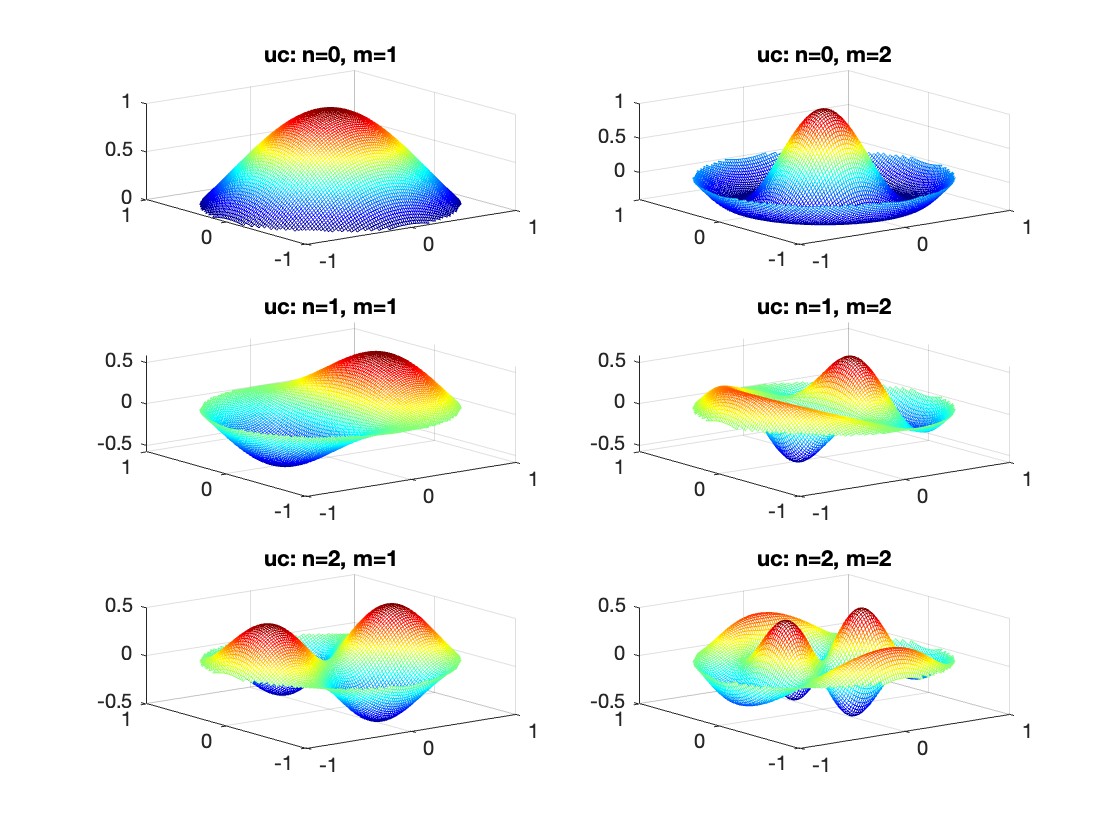
The following expression 

gives the solution for the Helmholtz problem. On the circular disc with center 0 and radius a. For  the plot in 3-dimensional graphics of the solutions on Matlab for
  and then calculate some eigenfunctions with the following expression.

It could be better to separate functions with  and
and  as follows
diska = 1; % Radius of the disk
mmax = 2; % Maximum value of m
nmax = 2; % Maximum value of n
% Function to find the k-th zero of the n-th Bessel function
% This function uses a more accurate method for initial guess
besselzero = @(n, k) fzero(@(x) besselj(n, x), [(k-(n==0))*pi, (k+1-(n==0))*pi]);
% Define the eigenvalue k[m, n] based on the zeros of the Bessel function
k = @(m, n) besselzero(n, m);
% Define the functions uc and us using Bessel functions
% These functions represent the radial part of the solution
uc = @(r, t, m, n) cos(n * t) .* besselj(n, k(m, n) * r);
us = @(r, t, m, n) sin(n * t) .* besselj(n, k(m, n) * r);
% Generate data for demonstration
data = zeros(5, 3);
for m = 1:5
for n = 0:2
data(m, n+1) = k(m, n); % Storing the eigenvalues
end
end
% Display the data
disp(data);
% Plotting all in one figure
figure;
plotIndex = 1;
for n = 0:nmax
for m = 1:mmax
subplot(nmax + 1, mmax, plotIndex);
[X, Y] = meshgrid(linspace(-diska, diska, 100), linspace(-diska, diska, 100));
R = sqrt(X.^2 + Y.^2);
T = atan2(Y, X);
Z = uc(R, T, m, n); % Using uc for plotting
% Ensure the plot is only within the disk
Z(R > diska) = NaN;
mesh(X, Y, Z);
title(sprintf('uc: n=%d, m=%d', n, m));
colormap('jet');
plotIndex = plotIndex + 1;
end
end

First, I felt that the three answers provided by a user in this thread might have been generated by AI. How do you think?
Second, I found that "Responsible usage of generative AI tools, such as ChatGPT, is allowed in MATLAB Answers."
If the answers are indeed AI generated, then the user didn't do "clearly indicating when AI generated content is incorporated".
That leads to my question that how do we enforce the guideline.
I am not against using AI for answers but in this case, I felt the answering text is mentioning all the relevant words but missing the point. For novice users who are seeking answers, this would be misleading and waste of time.
Mathworks has always had quality documentation but in 2023, the documentation quality fell. Will this improve in 2024?
Hi
I have Matlab 2015b installed and if I try:
ones(2,3,4)+ones(2,3)
of course I get an error. But my student has R2023b installed and she gets a 2x3x4 matrix as a result, with all elements = 2.
How is it possible?
Thanks
A

Can you solve it?
