Risultati per
We have created a new community for users of ThingSpeak. This new community is for students, researchers, and engineers looking to use MATLAB, Simulink, and ThingSpeak for Internet of Things applications. You can find the latest ThingSpeak news, tutorials to jump-start your next IoT project, and a forum to engage in a discussion on your latest cloud-based project. You can see answers to problems other users have solved and share how you solved a problem.
Christopher Stapels will be moderating the new ThingSpeak community .
We encourage you to visit the new community and share best practices, examples, and ask questions.
Happy New Year, everyone! We hope you enjoyed the Cody contest in 2020, learned new MATLAB skills, and made a friend or two. While the 2020 contest has concluded, the fun and learning never end.
Please take the 1-minute survey to talk about your experience (only 2 required questions). Our goal is to make future contests better and more appealing to you, so your feedback is critical to us.
Thank you in advance and hope to see you again in the 2021 contest.
Here's an example of virtualizing a lab course.
MathWorks is please to offer a new training course, Power Electronics Control Design with Simulink and Simscape.
This one-day course focuses on modeling and controlling power electronic systems in the Simulink® environment using Simscape Electrical™. Topics include:
- Modeling direct current (dc) power electronic components
- Controlling the level of fidelity in a model
- Developing controls for power electronics
- Modeling three-phase alternating current (ac) power electronic components
- Controlling power electronics for motor drive applications
Ameer Hamza had a great 2020 and has been awarded the coveted MOST ACCEPTED answers badge for all his contributions in MATLAB Answers this past year. Ameer joins Walter Roberson and Image Analyst in receiving this award going all the way back to 2012!
There are 10 community members who have achieved the Top Downloads badge for their popular File Exchange submissions in 2020. Do you recognize any of these names? There's a good chance you've used one or more of their toolboxes or scripts in your work if you're a frequent visitor to File Exchange, if you're not you might want to check out what they've posted, it may save you a lot of time writing your own code.
--------------------- Top Downloads Badge Winners -----------------
- PIRC
- Scott Lowe
- Yair Altman
- Dr. Siva Malla
- Chad Greene
- Seyedali Mirjalili
- Giampiero Campa
- Rodney Tan
- John D'Errico
- Steve Miller
Congratulations to all these winners and a giant THANK YOU for all they've done this past year to help everyone in the MATLAB Central community!
Hi everyone,
I am a third year BEng Energy Engineering student. I am looking at the design, modelling and peformance of an HVDC power converter for use in offshore wind for my final year dissertation. Power electronics is a new area for me and I am also new to simulink/ simscape elctrical.
Could anyone provide some useful examples of MMC (in particular rectifiers), or some advice for designing in simscape electrical. I am struggling with the design of PWM control especially. I aim to make a scaled down version of the MMC in Simulink but so far have had no luck. If anyone can help I would be really appreciative.
Thanks in advance.
Joe
Hi everybody!I've realized a DC/DC Buck Converter Model with closed loop control system. I need to limit the overshoot in the step response of the submitted system. I've already tried to tune the controller in the PID Tuner by manually adjusting the overshoot by moving the response time slider, as it is said in this article: https://it.mathworks.com/help/slcontrol/gs/automated-tuning-of-simulink-pid-controller-block.html The problem is that it is not accurate. I manage to get an overshoot of 4.77% or 5.4%, whereas i need to set the parameters in order that the overshoot is 5%. Should I use TuningGoal.Overshoot? How am I supposed to do? How should I set the input and output in my model? I've read Matlab documentation but I didn't catch that. Thanks in advance!
I am currently working on simulink online but I cannot maximize the screen
Just making sure people are aware of our new Onramp courses. These are great self-learning resources for students.
Released a few months ago:
Released this month:
Please I would be glad if I could be helped with the design of Microturbine coupled with PMSG.
How do you teach subjects like Programming and Numerical Computing hands-on in these challenging times?
Prof Chiranjoy Chattopadhyay at the Dept of Computer Science and Engineering at IIT Jodhpur shares his innovative approach to teaching at a distance in this new Technical Article on Teaching Parallel Computing Online with MATLAB.
The course utilized MATLAB Online , MATLAB Onramp and MATLAB Grader to train students in the basics of technical computing, in addition to using a Hands-on Online GPU workshop organised with the MathWorks Education Team. As a result of this approach to distance teaching, the students have reported good levels of understanding in the main learning outcomes of this course, as indicated in the survey results (below):
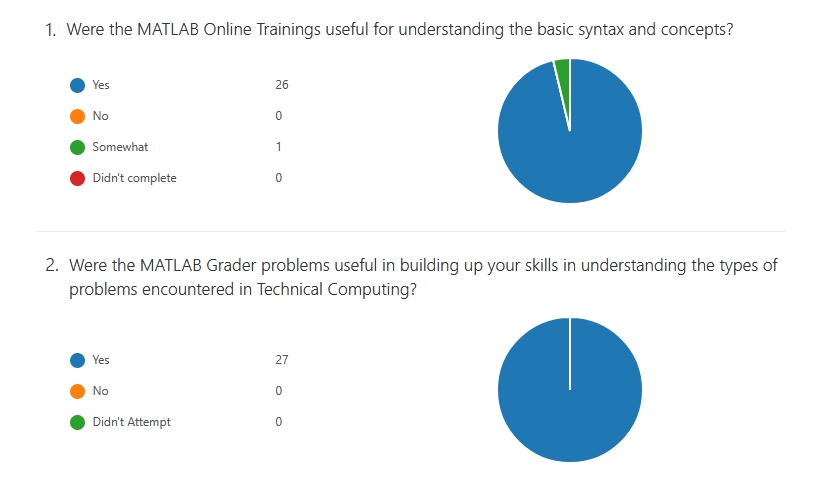
Please consider trying out the links above to check if your course might benefit from a similar approach, and feel free to message us if you are interested in learning more.
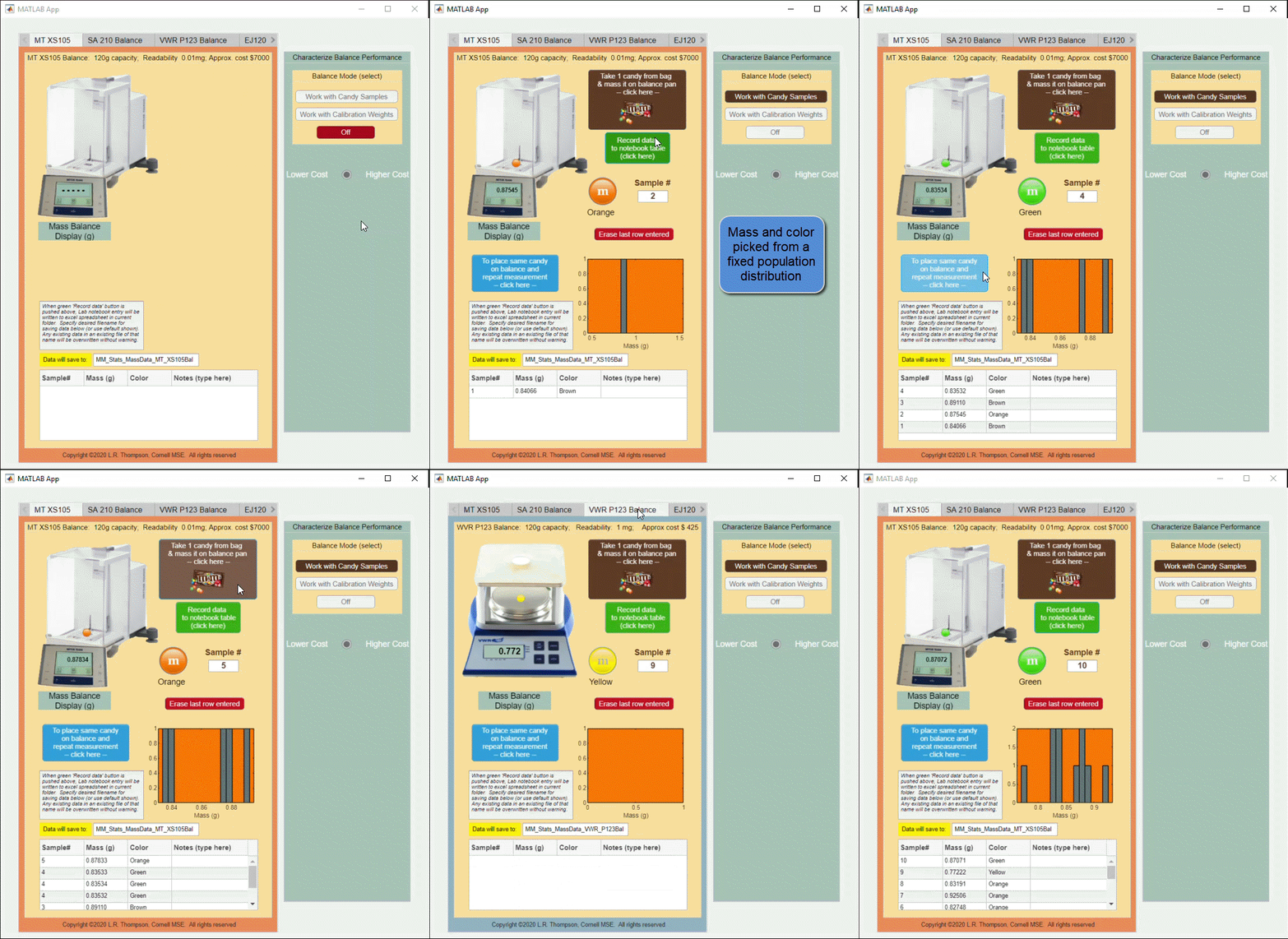
I just highlighted an app on File Exchange for emulating an experiment. Great idea for doing lab classes with software. What I like about this app is that it incorporates statistical variance and measurement noise that comes from physical experiments.
Read more about it here:
https://blogs.mathworks.com/pick/2020/11/20/emulating-a-physical-experiment-of-measuring-mms/
Hi everyone, I'm trying to estimate the Frequency Response of a buck converter. I've found this article: https://it.mathworks.com/company/newsletters/articles/estimating-the-frequency-response-of-a-power-electronics-model.html I've adapted the procedure to a buck converter and followed the instructions but something went wrong. In the last step I've performed a time-domain verification in a Simulink® simulation with the switch-mode buck converter and a Transfer Function block implementing the parametric estimation and compare the response of both systems to the same small perturbation signal but the estimated model response doesn't match the switching model response. I don't know why I've got a diverging systems. I've tried to reduce the load and modify the duty cycle but nothing changed. How can I fix it?
In the link below (File Exchange), you'll find an example with an electric motor supplied by a fuel cell stack (Simscape implementation) and a battery. When motor load is low-to-normal, the fuel cell provides excess energy, that is used to recharge the battery. At motor peak load, the battery needs to contribute in order to complete the expected duty. If you have any query or thoughts, please reach me at jsagardu@mathworks.com
https://www.mathworks.com/matlabcentral/fileexchange/59343-fuel-cell-battery-driven-electric-motor-h2-transfer
I would like to plot 2 discrete vectors on one graph created as follows: u=1; X={u,2*u,3*u,4*u,5*u,6*u,7*u,8*u,9*u}; Y={u,3*u,5*u,-u,-6*u,u-u,u^2,u^3,u^4}; stem(X,Y) unfortunately system returns error how to do it properly?
- Use the new exportapp function to capture an image of your app|uifigure
- MATLAB's getframe now supports apps & uifigures
- Review: How to get the handle to an app figure
Use the new exportapp function to capture an image of your app|uifigure
Imagine these scenarios:
- Your app contains several adjustable parameters that update an embedded plot and you'd like to remember the values of each app component so that you can recreate the plot with the same dataset
- You're constructing a manual for your app and would like to include images of your app
- You're app contains a process that automatically updates regularly and you'd like to store periodic snapshots of your app.
As of MATLABs R2020b release , we no longer must rely on 3rd party software to record an image of an app or uifigure.
exportapp(fig,filename) saves an image (JPEG | PNG | TIFF | PDF) of a uifigure ( fig) with the specified file name or full file path ( filename). MATLAB's documentation includes an example of how to add an [Export] button to an app that allows the user to select a path, filename, and extension for their exported image.
Here's another example that merely saves the image as a PDF to the app's main folder.
1. Add a button to the app and assign a ButtonPushed callback function to the button. This one also assigns an icon to the button in the form of an svg file.

2. Define the callback function to name the image after the app's name and include a datetime stamp. The image will be saved to the app's main folder.
% Button pushed function: SnapshotButton
function SnapshotButtonPushed(app, ~)
    % create filename containing the app's figure name (spaces removed)
    % and a datetime stamp in format yymmdd_hhmmss
    filename = sprintf('%s_%s.pdf',regexprep(app.MyApp.Name,' +',''), datestr(now(),'yymmdd_HHMMSS'));
    % Get the app's path
    filepath = fileparts(which([mfilename,'.mlapp']));
    % Store snapshot
    exportapp(app.MyApp, fullfile(filepath,filename))
end
Matlab's getframe now supports apps & uifigures
getframe(h) captures images of axes or a uifigure as a structure containing the image data which defines a movie frame. This function has been around for a while but as of r2020b , it now supports uifigures. By capturing consecutive frames, you can create a movie that can be played back within a Matlab figure (using movie ) or as an AVI file (using VideoWriter ). This is useful when demonstrating the effects of changes to app components.
The general steps to recording a process within an app as a movie are,
1. Add a button or some other event to your app that can invoke the frame recording process.
2. Animation is typically controlled by a loop with n iterations. Preallocate the structure array that will store the outputs to getframe. The example below stores the outputs within the app so that they are available by other functions within the app. That will require you to define the variable as a property in the app.
% nFrames is the number of iterations that will be recorded.
% recordedFrames is defined as a private property within the app
app.recordedFrames(1:nFrames) = struct('cdata',[],'colormap',[]);
3. Call getframe from within the loop that controls the animation. If you're using VideoWriter to create an AVI file, you'll also do that here (not shown, but see an example in the documentation ).
% app.myAppUIFigure: the app's figure handle
% getframe() also accepts axis handles
for i = 1:nFrames
... % code that updates the app for the next frame
      app.recordedFrames(i) = getframe(app.myAppUIFigure);
  end
4. Now the frame data are stored in app.recordedFrames and can be accessed from anywhere within the app. To play them back as a movie,
movie(app.recordedFrames)
% or
movie(app.recordedFrames, n) % to play the movie n-times
movie(app.recordedFrames, n, fps) % to specify the number of frames per second
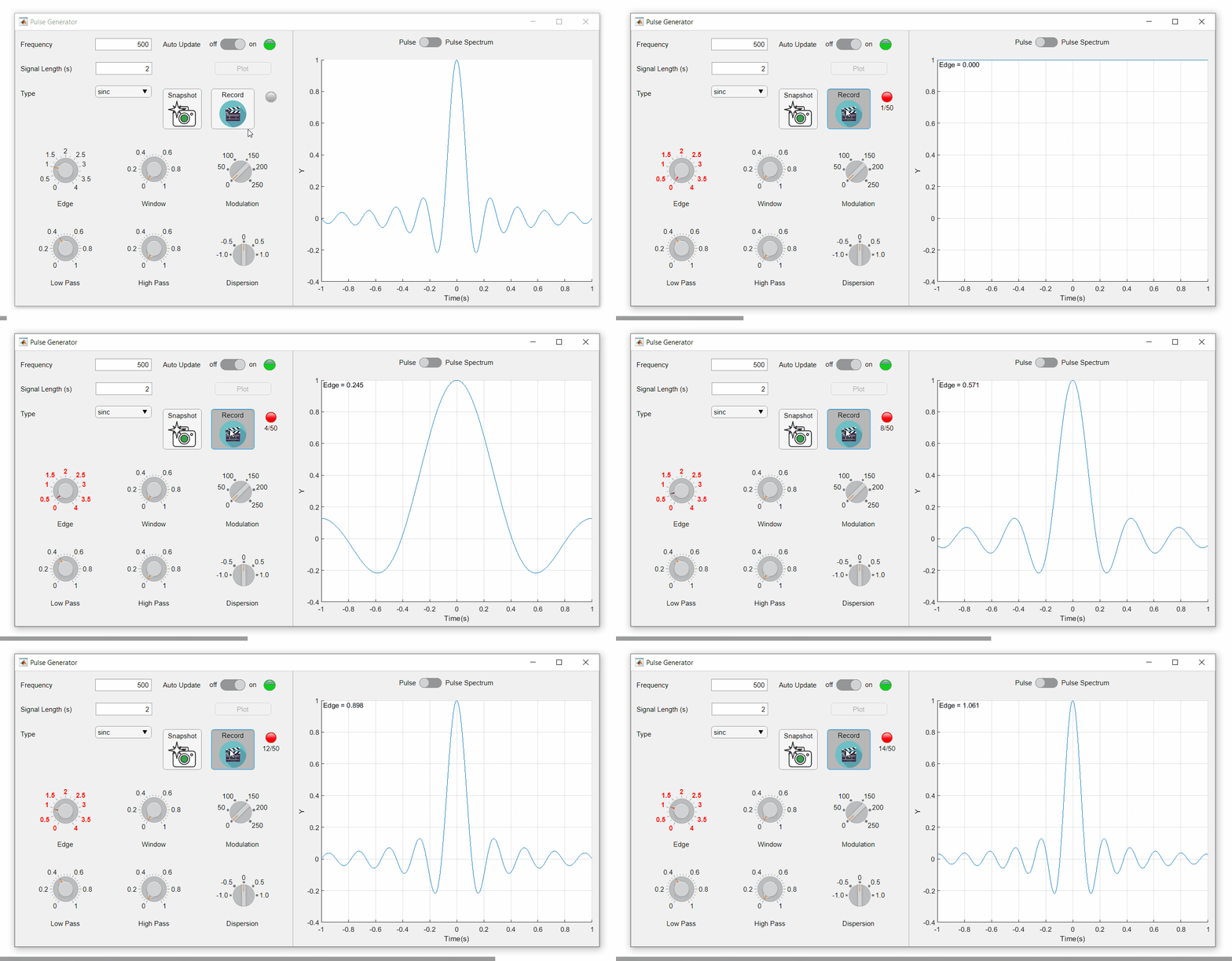
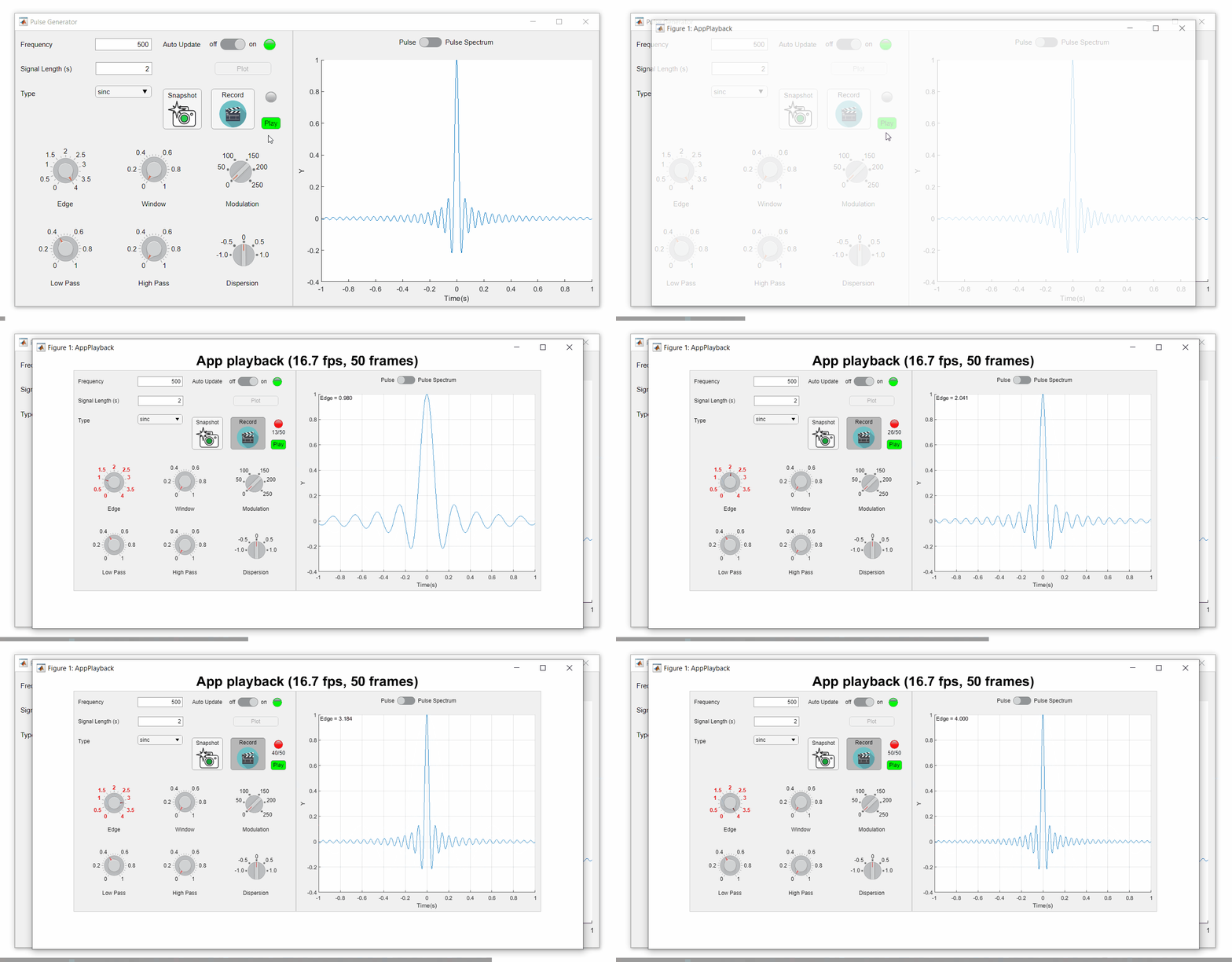
To demonstrate this, I adapted a copy of Matlab's built-in PulseGenerator.mlapp by adding
- a record button
- a record status lamp with frame counter
- a playback button
- a function that animates the effects of the Edge Knob
Recording process (The GIF is a lot faster than realtime and only shows part of the recording) (Open the image in a new window or see the attached Live Script for a clearer image).
Playback process (Open the image in a new window or see the attached Live Script for a clearer image.)
Review: How to get the handle to an app figure
To use either of these functions outside of app designer, you'll need to access the App's figure handle. By default, the HandleVisibility property of uifigures is set to off preventing the use of gcf to retrieve the figure handle. Here are 4 ways to access the app's figure handle from outside of the app.
1. Store the app's handle when opening the app.
app = myApp;
% Get the figure handle
figureHandle = app.myAppUIFigure;
2. Search for the figure handle using the app's name, tag, or any other unique property value
allfigs = findall(0, 'Type', 'figure'); % handle to all existing figures
figureHandle = findall(allfigs, 'Name', 'MyApp', 'Tag', 'MyUniqueTagName');
3. Change the HandleVisibility property to on or callback so that the figure handle is accessible by gcf anywhere or from within callback functions. This can be changed programmatically or from within the app designer component browser. Note, this is not recommended since any function that uses gcf such as axes(), clf(), etc can now access your app!.
4. If the app's figure handle is needed within a callback function external to the app, you could pass the app's figure handle in as an input variable or you could use gcbf() even if the HandleVisibility is off.
See a complete list of changes to the PulseGenerator app in the attached Live Script file to recreate the app.
File Exchange now offers the ability to download/restore previous versions of community contributed files. It's often a good practice to always update your software to the latest version, however there are times when this isn't always helpful. Sometimes a software update can break or alter something you've been relying on, in these cases you'll want to stick with the version that's working for you. This is why we've added the ability to download previous versions in File Exchange.
Using Version History
Navigate to any community member file and then click the View Version History link that appears above the Download button. This will show you a list of the previous versions contributed by the submission author. Each version will have a corresponding download button, date, version number, and a description of the changes made for that update.
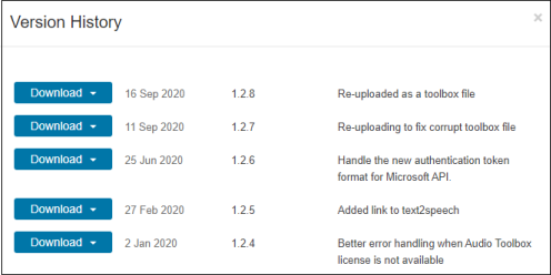
Let us know what you think about this new feature by replying below.
Here's a short article describing how educators from UNSW have used Live Scripts to help students understand mathematical models. Interactive live scripts allow students to experiment and understand concepts through trial and error. The article also explains how the scripts helped provide an enriched online learning experience for the students.
Do you use Live Scripts in your teaching?
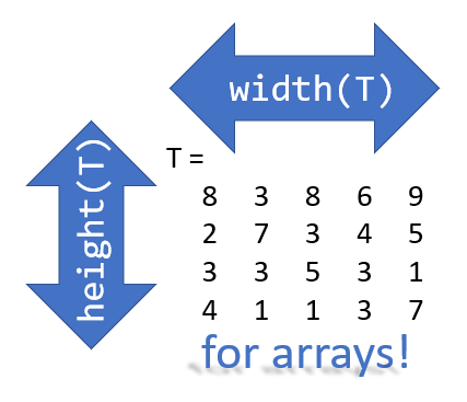
Prior to r2020b the height (number of rows) and width (number of columns) of an array or table can be determined by the size function,
array = rand(102, 16);
% Method 1
[dimensions] = size(array);
h = dimensions(1);
w = dimensions(2);
% Method 2
[h, w] = size(array); %#ok<*ASGLU>
% or
[h, ~] = size(array);
[~, w] = size(array);
% Method 3
h = size(array,1);
w = size(array,2);
In r2013b, the height(T) and width(T) functions were introduced to return the size of single dimensions for tables and timetables.
Starting in r2020b, height() and width() can be applied to arrays as an alternative to the size() function.
Continuing from the section above,
h = height(array)
% h =  102
w = width(array)
% w =  16
height() and width() can also be applied to multidimensional arrays including cell and structure arrays
mdarray = rand(4,3,20);
h = height(mdarray)
% h =  4
w = width(mdarray)
% w =  3
The expanded support of the height() and width() functions means,
- when reading code, you can no longer assume the variable T in height(T) or width(T) refers to a table or timetable
- greater flexibility in expressions such as the these, below
% C is a 1x4 cell array containing 4 matrices with different dimensions
rng('default')
C = {rand(5,2), rand(2,3), rand(3,4), rand(1,1)};
celldisp(C)
% C{1} =
%       0.81472      0.09754
%       0.90579       0.2785
%       0.12699      0.54688
%       0.91338      0.95751
%       0.63236      0.96489
% C{2} =
%       0.15761      0.95717      0.80028
%       0.97059      0.48538      0.14189
% C{3} =
%       0.42176      0.95949      0.84913      0.75774
%       0.91574      0.65574      0.93399      0.74313
%       0.79221     0.035712      0.67874      0.39223
% C{4} =
%       0.65548
What's the max number of rows in C?
maxRows1 = max(cellfun(@height,C))         % using height()
% maxRows1 =  5;
maxRows2 = max(cellfun(@(x)size(x,1),C))   % using size()
% maxRows2 =  5;
What's the total number of columns in C?
totCols1 = sum(cellfun(@width,C))          % using width()
%totCols1 =  10
totCols2 = sum(cellfun(@(x)size(x,2),C))   % using size(x,2)
% totCols2 =  10
Attached is a live script containing the content of this post.
Hi All,
Using the PMLSM SimScape block for my FOC PMLSM model - PMLSM
In the example ee_pmlsm_drive.slx which i have based my FOC architedure on, have a few questions please.
There is a gain block after the outer loop velocity controller (iq_Ref), which is the inverse of the Force constant (Kt) shown as (2/3*Np*PM) in the literature. This is also used in the PMSM FOC model, placed after the torque limiter Tq to iq_Ref. Why is this inverse Kt gain added to the idq_ref signal? Does this cancel Kt if its used in the Force Equation?
Previous help posts regarding the Force Constant (Kt), imply emitting the constant (3/2) in Kt. Also in the PMLSM help center document states Ke, Kt and Flux linkage are equal. Does this simplification apply to the translational machine counterpart SimScape block?
I have tried to look into the SimScape block code of the PMLSM to confirm, how do i look under the mask to check the Force equation for the PMLSM to confirm Kt and Ke used in this model?
Any help would be great as this is holding up Validation of my "small signal" linear PMLSM model against the SimScape PMLSM block model.
Thanks
Patrick
