Estimating Risk-Neutral Density from Option Prices with a MATLAB App

Because over-the-counter options contracts are sold by one private party to another rather than on the open market, it can be difficult to determine whether an agreed-upon price favors the buyer or the seller. To price these contracts, financial analysts often rely on risk-neutral density (RND) estimates inferred from observed call and put option prices. It is common practice to calculate RND estimates using a pricing model with parameter values based on historical market data.

Relying on parametric pricing models to estimate RND has several drawbacks, including long processing times and potential biases. Simple models can be calibrated faster, but they tend to be inconsistent with some of the empirical properties characterizing financial data, producing highly biased results, while more sophisticated models designed for better accuracy may take a long time to calibrate—typically hours when no closed-form solutions are available. Even sophisticated models can deliver results that look reasonable but may, in fact, be biased due to the use of an inefficient numerical technique. In addition, because pricing models depend heavily on historical data, it is up to the developer to decide how much data to include—a subjective decision that can influence the results.

Our research team at Aarhus University has developed a non-structural, model-free methodology for estimating RND that does not rely on a parametric model but lets the data speak for itself. The methodology uses orthogonal polynomial expansions to estimate RND and options greeks from current rather than historical data, and it produces results much faster than model-driven approaches—the typical duration of an RND estimate is a few seconds.

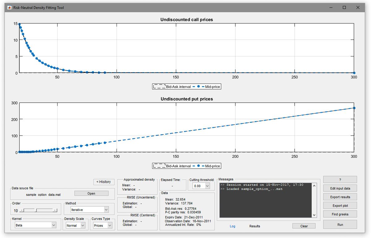
To demonstrate our methodology and make it easier for students, analysts, and researchers to apply, we packaged it as a MATLAB^® app (Figure 1). The Risk-Neutral Density Fitting Tool app complements the approach detailed in our papers A Non-Structural Investigation of VIX Risk Neutral Density (estimation of RND) and It Only Takes a Few Moments to Hedge (estimation of greeks).

Why We Chose MATLAB

We decided to create a MATLAB app for RND estimation because we wanted to make our research widely accessible rather than restrict its use to quantitative economics and finance researchers who are experienced MATLAB programmers.

We found that MATLAB dramatically increased our development speed. We completed most of the development in two to three months—we estimate that it would have taken us about two years using a traditional compiled language. Because MATLAB is an interpreted language and runs on a JIT compiler, we avoided cumbersome edit-compile-test cycles; instead, we developed our methodology interactively, invoking functions in MATLAB and iteratively examining the results. And rather than relying on third-party libraries or writing our own algorithms for linear regression, principal component analysis, and other capabilities, we took advantage of verified functions from Curve Fitting Toolbox™, Financial Toolbox™, Optimization Toolbox™, and Statistics and Machine Learning Toolbox™. Performance can be a concern when using interpreted languages. However, by making use of the vectorized operations and optimized functions in MATLAB, we achieved performance close to that of a compiled language.

Beyond accelerating the implementation of our RND methodology, MATLAB made it easy to build the interface and package it with the underlying code as an app. We used MATLAB application development tools to design the windows, buttons, and other controls in the interface. We then packaged the complete app into a single installer file that we made available for download on the project’s GitHub page.

Estimating RND and Finding the Greeks with the App

Once the app has been downloaded and installed, a typical workflow begins with loading option price data from a source such as OptionMetrics or the Chicago Board Options Exchange (Cboe), both natively supported by the app. Next, the user examines the price curves for the input data and optionally adjusts strike boundaries (the minimum and maximum price at which put or call options are exercised). The user then selects the kernel, the expansion order, and the method to be used to estimate the expansion coefficients (for example, principal component analysis). The kernel specifies the probability distribution to be used as initial proxy for the true RND, whereas the expansion order defines the number of orthogonal polynomials that “correct” the kernel to approximate the RND.

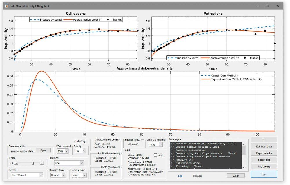
The app has several built-in kernels, including beta gamma, generalized inverse Gaussian, generalized Weibull, and lognormal, and it can be extended with custom kernels written as MATLAB functions. A higher expansion order leads to a more precise expansion but will generally require more time to compute the estimate (Figure 2).

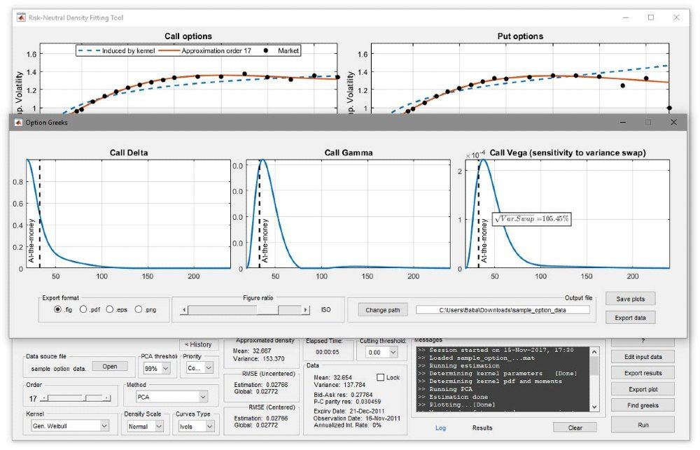
Finally, to compute the delta, gamma, and vega sensitivities, the user simply clicks the app’s “Find Greeks” button. Plots of these three sensitivities are generated and displayed in the interface (Figure 3).

All plots can be saved as MATLAB figures or as PNG, PDF, or EPS files, and all results can be exported and saved for further analysis.

Future Enhancements

The feedback we have received from users of the app has been quite positive. We are using this feedback to improve the app and plan future enhancements. For example, we are considering adding time and maturity dimensions to the analysis, and we are exploring the use of multivariate densities as well as the possibility of forecasting an entire density curve from using historical observations of option prices instead of curves observed at a single point in time.

Acknowledgement

The development of this app received funding from the Danish Council for Independent Research as part of the research project The Invisible Risks of Derivatives Valuation Models (DFF – 6109-00056).

Aarhus University is among the nearly 1000 universities worldwide that provide campus-wide access to MATLAB and Simulink^®. With the Total Academic Headcount (TAH) License, researchers, faculty, and students have access to a common configuration of products, at the latest release level, for use anywhere—in the classroom, at home, in the lab, or in the field.