Train Image Classification Network Robust to Adversarial Examples
This example shows how to train a neural network that is robust to adversarial examples using fast gradient sign method (FGSM) adversarial training.
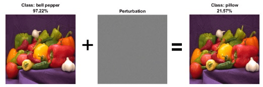
Neural networks can be susceptible to a phenomenon known as adversarial examples [1], where very small changes to an input can cause it to be misclassified. These changes are often imperceptible to humans.
Techniques for creating adversarial examples include the FGSM [2] and the basic iterative method (BIM) [3], also known as projected gradient descent [4].
You can use adversarial training [5] to train networks that are robust to adversarial examples. This example shows how to:
Train an image classification network.
Investigate network robustness by generating adversarial examples.
Train an image classification network that is robust to adversarial examples.
Load Training Data
The digitTrain4DArrayData function loads images of handwritten digits and their labels.
rng("default")
[XTrain,TTrain] = digitTrain4DArrayData;
Extract the class names.
classNames = categories(TTrain);
numObservations = numel(TTrain);
Use the trainingPartitions function to split the data into training and validation sets. This function is attached as a supporting file. To access the function, open the example.
[idxTrain,idxValidation] = trainingPartitions(numObservations,[0.85 0.15]);

XValidation = XTrain(:,:,:,idxValidation);
TValidation = TTrain(idxValidation);

XTrain = XTrain(:,:,:,idxTrain);
TTrain = TTrain(idxTrain);
Construct Network Architecture
Create a convolutional neural network suitable for image classification.
layers = [
    imageInputLayer([28 28 1])

    convolution2dLayer(3,8,Padding="same")
    batchNormalizationLayer
    reluLayer

    maxPooling2dLayer(2,Stride=2)

    convolution2dLayer(3,16,Padding="same")
    batchNormalizationLayer
    reluLayer

    maxPooling2dLayer(2,Stride=2)

    convolution2dLayer(3,32,Padding="same")
    batchNormalizationLayer
    reluLayer

    fullyConnectedLayer(10)
    softmaxLayer];
Specify the training options. Choosing among the options requires empirical analysis. To explore different training option configurations by running experiments, you can use the Experiment Manager app.
optionsTrainNetwork = trainingOptions("sgdm", ...
    InitialLearnRate=0.01, ...
    MaxEpochs=5, ...
    Shuffle="every-epoch", ...
    ValidationData={XValidation,TValidation}, ...
    Plots="training-progress", ...
    Metrics="accuracy", ...
    Verbose=false);
Train the network using the trainnet function.
net = trainnet(XTrain,TTrain,layers,"crossentropy",optionsTrainNetwork);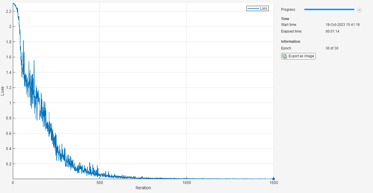
Test Network
Test the classification accuracy of the network by evaluating network predictions on a test data set. Make predictions using the minibatchpredict function, and convert the classification scores to labels using the scores2label function.
[XTest,TTest] = digitTest4DArrayData;

scores = minibatchpredict(net,XTest);
YTest = scores2label(scores,classNames);

accuracy = mean(YTest == TTest)
accuracy =
0.9754
The network accuracy is very high.
Generate Adversarial Examples
Apply adversarial perturbations to the input images and see how doing so affects the network accuracy.
You can generate adversarial examples using techniques such as FGSM. FGSM is a simple technique that takes a single step in the direction of the gradient of the loss function , with respect to the image you want to find an adversarial example for. The adversarial example is calculated as
.
Parameter is the step size and controls how different the adversarial examples look from the original images. In this example, the values of the pixels are between 0 and 1, so an value of 0.01 alters each individual pixel value by up to 1% of the range. The value of depends on the image scale. For example, if your image is instead between 0 and 255, you need to multiply this value by 255.
BIM is a simple improvement to FGSM which applies FGSM over multiple iterations and applies a threshold. This method can yield adversarial examples with less distortion than FGSM. For more information about generating adversarial examples, see Generate Untargeted and Targeted Adversarial Examples for Image Classification. Create adversarial examples using the BIM.
Create lower and upper bounds using the test data.
epsilon = 0.1;

XLowerTest = dlarray(max(XTest-epsilon,0),"SSCB");
XUpperTest = dlarray(min(XTest+epsilon,1),"SSCB");
Define the step size and the number of iterations using the adversarialOptions function.
alpha = 0.01;
numAdvIter = 20;

optionsAdversarialTest = adversarialOptions("bim",NumIterations=numAdvIter,StepSize=alpha);
Use the findAdversarialExamples function to generate adversarial examples.
[examplesTest,mislabelsTest,iXTest] = findAdversarialExamples(net,XLowerTest,XUpperTest,TTest,Algorithm=optionsAdversarialTest);
trueLabelsTest = TTest(iXTest);
View the original image and the adversarial example side-by-side. The adversarial example is misclassified even though the adversarial image appears very similar to the original image.
figure
tiledlayout(1,3);

nexttile;
imshow(XTest(:,:,:,iXTest(1)));
title({"Original Image","Label: " + string(trueLabelsTest(1))});

nexttile
imshow(1-(extractdata(examplesTest(:,:,:,1)) - XTest(:,:,:,iXTest(1))));
title("Perturbation")

nexttile
imshow(extractdata(examplesTest(:,:,:,1)));
title({"Adversarial Example", "Label: " + string(mislabelsTest(1))});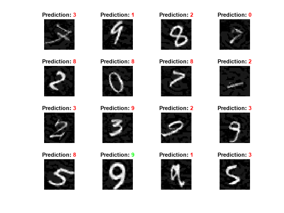
Train Robust Network
You can train a network to be robust against adversarial examples. One popular method is adversarial training. Adversarial training involves finding adversarial examples and adding them to the training set.
Generate a new set of adversarial examples to add to the training data. For the network to be robust to perturbations of size , perform FGSM training with a value slightly larger than . For this example, perturb the training images using step size .
XLowerTrain = dlarray(max(XTrain-epsilon,0),"SSCB");
XUpperTrain = dlarray(min(XTrain+epsilon,1),"SSCB");

optionsAdversarialTrain = adversarialOptions("fgsm",StepSize=1.25*epsilon);

[examplesTrain,~,iXTrain] = findAdversarialExamples(net,XLowerTrain,XUpperTrain,TTrain,Algorithm=optionsAdversarialTrain);
trueLabelsTrain = TTrain(iXTrain);
Augment the training data set with the new adversarial examples.
augmentedXTrainData = cat(4,XTrain,examplesTrain);
augmentedTTrainData = cat(1,TTrain,trueLabelsTrain);
Train the network on the original and the adversarial data.
netRobust = trainnet(augmentedXTrainData,augmentedTTrainData,layers,"crossentropy",optionsTrainNetwork);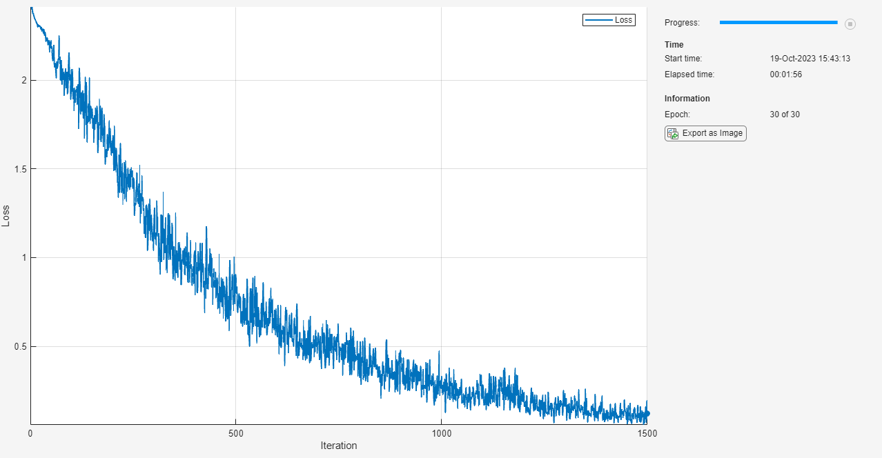
Test the classification accuracy of the robust network by evaluating network predictions on the original test data set. The robust network still performs well on the original test set.
scoresRobust = minibatchpredict(netRobust,XTest);
YTestRobust = scores2label(scoresRobust,classNames);

accuracy = mean(YTestRobust == TTest)
accuracy =
0.9832
Compare Robust and Nonrobust Networks on Adversarial Examples
Compute the accuracy of the nonrobust and the robust network on the adversarial example data.
scoresTestAdv = minibatchpredict(net,examplesTest);
YTestAdv = scores2label(scoresTestAdv,classNames);
accuracyAdv = mean(YTestAdv == trueLabelsTest')
accuracyAdv =
0
scoresTestAdvRobust = minibatchpredict(netRobust,examplesTest);
YTestAdvRobust = scores2label(scoresTestAdvRobust,classNames);
accuracyRobustTest = mean(YTestAdvRobust == trueLabelsTest')
accuracyRobustTest =
0.9796
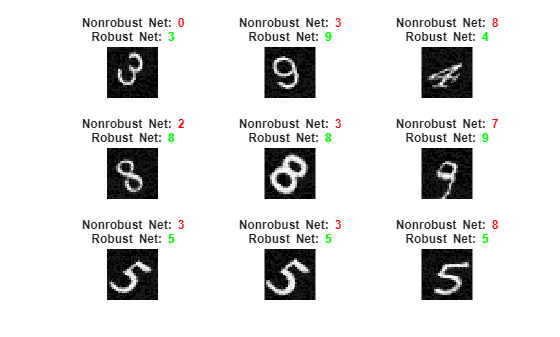
Plot the results. You can see that for the original network, the accuracy is severely degraded for the adversarial examples. However, the robust network still accurately classifies the images.
visualizePredictions(examplesTest,YTestAdv,YTestAdvRobust,trueLabelsTest);
Supporting Functions
Visualize images along with their predicted classes. Correct predictions use green text. Incorrect predictions use red text.
function visualizePredictions(XTest,YPred,YPredAdv,TTest)

figure
height = 3;
width = 3;
numImages = height*width;

% Select random images from the data.
indices = randperm(size(XTest,4),numImages);

XTest = extractdata(XTest);
XTest = XTest(:,:,:,indices);
YPred = YPred(indices);
YPredAdv = YPredAdv(indices);
TTest = TTest(indices);

% Plot images with the predicted label.
for i = 1:(numImages)
    subplot(height,width,i)
    imshow(XTest(:,:,:,i))

    % If the prediction is correct, use green. If the prediction is false,
    % use red.
    if YPred(i) == TTest(i)
        color = "\color{green}";
    else
        color = "\color{red}";
    end

    if YPredAdv(i) == TTest(i)
        colorAdv = "\color{green}";
    else
        colorAdv = "\color{red}";
    end

    title({"Nonrobust Net: " + color + string(YPred(i)), ...
        "Robust Net: " + colorAdv + string(YPredAdv(i))})
end

end
References
[1] Szegedy, Christian, Wojciech Zaremba, Ilya Sutskever, Joan Bruna, Dumitru Erhan, Ian Goodfellow, and Rob Fergus. “Intriguing Properties of Neural Networks.” Preprint, submitted February 19, 2014. https://arxiv.org/abs/1312.6199.
[2] Goodfellow, Ian J., Jonathon Shlens, and Christian Szegedy. “Explaining and Harnessing Adversarial Examples.” Preprint, submitted March 20, 2015. https://arxiv.org/abs/1412.6572.
[3] Kurakin, Alexey, Ian Goodfellow, and Samy Bengio. “Adversarial Examples in the Physical World.” Preprint, submitted February 10, 2017. https://arxiv.org/abs/1607.02533.
[4] Madry, Aleksander, Aleksandar Makelov, Ludwig Schmidt, Dimitris Tsipras, and Adrian Vladu. “Towards Deep Learning Models Resistant to Adversarial Attacks.” Preprint, submitted September 4, 2019. https://arxiv.org/abs/1706.06083.
[5] Wong, Eric, Leslie Rice, and J. Zico Kolter. “Fast Is Better than Free: Revisiting Adversarial Training.” Preprint, submitted January 12, 2020. https://arxiv.org/abs/2001.03994.
See Also
dlfeval | dlnetwork | dlgradient | arrayDatastore | minibatchqueue | estimateNetworkOutputBounds | verifyNetworkRobustness
Topics
- Verification of Neural Networks
- Generate Untargeted and Targeted Adversarial Examples for Image Classification
- Generate Adversarial Examples for Semantic Segmentation
- Verify Robustness of Deep Learning Neural Network
- Define Model for Custom Training Loop
- Grad-CAM Reveals the Why Behind Deep Learning Decisions
- Out-of-Distribution Detection for Deep Neural Networks
- Verify an Airborne Deep Learning System