Fixed-Point Tool
Convert a floating-point model to a fixed-point model
Description
The Fixed-Point Tool enables you to automatically convert a floating-point model to use fixed-point data types, optimize existing data types on a model, and analyze ranges and data types on your model using rich statistics and visualizations.
The Fixed-Point Tool provides three workflows for data type conversion and analysis depending on your needs:
Optimized Fixed-Point Conversion — Automatically convert your model to use optimized fixed-point data types.
Iterative Fixed-Point Conversion — Automatically propose fixed-point data types and manually select which data types to apply to your model.
Range Collection — Explore the numerical behavior of your model before or after data type conversion.
The table below provides a summary of the differences between these three workflows. Data Type Conversion Overview explains these options in more detail.
| Workflow | Changes Model Data Types | Ease of Use | Amount of Control Over Data Types Applied to Model | Requires Knowledge of System Behavior Tolerances | Command-Line Workflow |
|---|---|---|---|---|---|
| Optimized Fixed-Point Conversion | Yes | One step | Low | Yes | fxpopt |
| Iterative Fixed-Point Conversion | Yes | Multiple iterations | High | Recommended | DataTypeWorkflow.Converter |
| Range Collection | No | One step | N/A | Recommended |

Open the Fixed-Point Tool
Simulink® Toolstrip: On the Apps tab, under Code Generation, click the app icon.
MATLAB® command prompt: Enter
fxptdlg('system_name'), where'system_name'is the name of the model or system you want to convert, specified as a string.
Examples
This example shows how to use the Optimized Fixed-Point Conversion workflow in the Fixed-Point Tool. The model used in this example is a simple FIR filter modeled using floating-point data types. In this example, you specify known behavioral constraints for the output of the filter and optimize the fixed-point data types in the Embedded Efficient Filter subsystem.
Open the mSimpleFIR model.
open_system('mSimpleFIR');

Inspect the Embedded Efficient Filter subsystem.
open_system('mSimpleFIR/Embedded Efficient Filter');

Known design minimum and maximum values are specified explicitly on blocks in the model, including on the inputs and outputs of the Embedded Efficient Filter subsystem.
Open the Fixed-Point Tool. On the Simulink® Apps tab, under Code Generation, click the app icon.
To start the optimized fixed-point conversion workflow, select Optimized Fixed-Point Conversion.
Select the subsystem that you want to analyze. Under System Under Design (SUD), select the Embedded Efficient Filter subsystem.
Choose the range collection method to use. Under Range Collection Mode, select Simulation with derived ranges. During the range analysis step of optimization, the tool will combine ranges from simulation minimum and maximum values, design minimum and maximum values specified explicitly on blocks in the model, and derived minimum and maximum values that are computed through a static analysis that derives ranges for objects in the model.
Specify Simulation Inputs. For this example, use the default model inputs for simulation.
Specify signal tolerances for logged signals. Set the Absolute Tolerance and Relative Tolerance of the output_signal:1 to 0.01.

To prepare the model for fixed-point conversion, click Prepare. The Fixed-Point Tool creates a backup version of the model and checks the model for compatibility with the conversion process. For more about preparation checks, see Use the Fixed-Point Tool to Prepare a System for Conversion.

Next, expand the Optimization Options button arrow to configure the options to use for data type optimization. For this example, use the default.

To optimize data types in the model, click Optimize Data Types.
During the optimization process, the software analyzes ranges of objects in your system under design. Optimization will take into account all specified behavioral constraints, including design minimum and maximum values and signal tolerances, to apply heterogeneous data types to your system while minimizing the objective function. For this example, the objective function is set to the default Bit Width Sum, which instructs the optimization to minimize the sum of word lengths in the system under design.
During the optimization process, the software makes changes to several settings and model configuration parameters. The purposes of these changes include suppressing diagnostics, enabling logging with the Simulation Data Inspector, reducing the memory consumed by the result, ensuring validity of the model, accelerating the optimization process, and turning off data type override. For more information, see Model Configuration Changes Made During Data Type Optimization. You can restore these diagnostics after the optimization is complete.
Details about the optimization process are printed to the Optimization Details pane in the Fixed-Point Tool. You can pause or stop the optimization solver before the optimization search is complete by clicking Stop.

When the optimization is complete, the Fixed-Point Tool displays a table that contains all of the solutions found during the optimization process. Solution 1 in the table corresponds to the best solution found.
Solutions are ordered in the table based on the Cost, which is defined by the objective function specified in the Optimization Options menu. Feasible solutions that meet the defined behavioral constraints are marked with a pass status in the solutions table. Solutions that do not meet the behavioral constraints are marked with a fail status. The solutions are also plotted in a scatter chart that compares the cost and maximum difference of each solution to help you visualize the tradeoff between accuracy and cost-efficiency for each solution. When you select any solution in the table, the solution is highlighted in the scatter chart.
This example uses tolerances on the output of the filter subsystem to define the desired behavior of the system. For more information about defining other types of behavioral constraints, see Specify Behavioral Constraints.

During the optimization process, the tool collects ranges and statistics for objects in your model. To explore these ranges, in the Workflow Browser pane, select BaselineRun.

The Results spreadsheet displays a summary of the statistics collected during the range collection phase of optimization, including simulation minimum and simulation maximum values. You can click any result to view additional details in the Result Details pane. The Visualization of Simulation Data pane displays a summary of histograms of the bits used by each object in your model.
You can customize the information displayed in the Results spreadsheet, or use the Explore tab to sort and filter these results based on additional criteria. For more information, see Control Views in the Fixed-Point Tool.
The best solution found during optimization, Solution 1, is automatically applied to the model. To compare this optimized solution to the baseline run, click Compare. In the Embedded Efficient Filter subsystem, you can see the applied optimized fixed-point data types. When you click Compare for a model that has logged signals, the tool opens the Simulation Data Inspector. In the Simulation Data Inspector, select output_signal as the signal to compare. The plot of the plant output signal for Solution 1 is within the specified tolerance band.

You can continue exploring other solutions by selecting a solution from the solutions table and clicking Apply and Compare.
After optimizing data types in the Fixed-Point Tool, you can choose to export the optimization workflow steps to a MATLAB® script. This allows you to save the current optimization workflow steps and continue data type optimization using fxpopt at the command line.
Click Export Script to export a script named fxpOptimizationOptions to the current working directory.
After the conversion process, if you want to restore your model to its state at the start of the conversion process, click Restore Original Model. Any changes made to your model after the preparation stage of conversion are removed.
This example shows how to use the Iterative Fixed-Point Conversion workflow in the Fixed-Point Tool. The model used in this example is a simple FIR filter modeled using initial guesses for fixed-point data types. In this example, you specify known behavioral constraints for the output of the filter and improve the fixed-point data types in the Embedded Efficient Filter subsystem.
Open the mSimpleFIR_fxp model.
open_system('mSimpleFIR_fxp');

Inspect the Embedded Efficient Filter subsystem.
open_system('mSimpleFIR_fxp/Embedded Efficient Filter');

Known design minimum and maximum values are specified explicitly on blocks in the model, including on the inputs and outputs of the Embedded Efficient Filter subsystem.
Open the Fixed-Point Tool. On the Simulink® Apps tab, under Code Generation, click the app icon.
To start the iterative fixed-point conversion workflow, select Iterative Fixed-Point Conversion.
Select the subsystem that you want to analyze. Under System Under Design (SUD), select the Embedded Efficient Filter subsystem.
Choose the range collection method to use. Under Range Collection Mode, select Simulation with derived ranges. During the range analysis step of optimization, the tool will combine ranges from simulation minimum and maximum values, design minimum and maximum values specified explicitly on blocks in the model, and derived minimum and maximum values that are computed through a static analysis that derived ranges for objects in the model.
Specify Simulation Inputs. For this example, use the default model inputs for simulation.
Specify signal tolerances for logged signals. Set the Absolute Tolerance and Relative Tolerance of the output_signal:1 to 0.01.

To prepare the model for fixed-point conversion, click Prepare. The Fixed-Point Tool creates a backup version of the model and checks the model for compatibility with the conversion process. For more about preparation checks, see Use the Fixed-Point Tool to Prepare a System for Conversion.

Next, collect ranges. Expand the Collect Ranges button arrow and select Double precision. Click Collect Ranges to start the range collection run.

When you select Double precision as the range collection mode, the tool simulates the system under design with data type override enabled. Data type override performs a global override of the fixed-point data types in the model, thereby avoiding quantization effects. This enables you to establish an ideal floating-point baseline for the behavior of your model.

The results of range collection are stored in BaselineRun. The Results spreadsheet displays a summary of the statistics collected during the range collection simulation, including the currently specified data types on the model (SpecifiedDT), simulation minimum, and simulation maximum values. The compiled data type (CompiledDT) column displays double for all objects in the Embedded Efficient Filter subsystem, indicating that data type override was applied during the range collection simulation.
You can click on any result to view additional details in the Result Details pane. The Visualization of Simulation Data pane displays a summary of histograms of the bits used by each object in your model. The simulation data shows that several objects in the model have potential underflows.
You can customize the information displayed in the Results spreadsheet, or use the Explore tab to sort and filter these results based on additional criteria. For more information, see Control Views in the Fixed-Point Tool.
Next, expand the Settings button arrow to configure the settings to use for data type proposals. Set Propose to Word Length.

To propose data types based on the ranges collected and the data type proposal settings specified, click Propose Data Types. The tool uses all available range data to calculate data type proposals which can include design minimum or maximum values, simulation minimum or maximum values, and derived minimum or maximum values. Data types are proposed for all objects in the system under design whose Lock output data type setting against changes by the fixed-point tools parameter is cleared.

To write the proposed data types to the model, click Apply Data Types. The tool updates the SpecifiedDT column to show that the data types have been applied to the model.
Simulate the model using the applied fixed-point data types. Expand the Simulate with Embedded Types button arrow and select Specified data types. Then click Simulate with Embedded Types.
The Fixed-Point Tool simulates the model using the new fixed-point data types and logs minimum and maximum values and overflow data for all objects in the system under design. This information is stored in a new run named EmbeddedRun. The icon next to EmbeddedRun displays a pass status, indicating that all signals in the system under design meet the specified tolerances. The Visualization of Simulation Data pane updates to display the new EmbeddedRun data.

To compare the ideal results stored in BaselineRun with the newly applied fixed-point data types, select EmbeddedRun from the Run to compare in SDI drop down menu. Then click Compare Results to open the Simulation Data Inspector.
In the Simulation Data Inspector, select output_signal as the signal to compare.

The plot of the filter output signal for EmbeddedRun is within the specified tolerance band.
If the behavior of the converted system does not meet your requirements or if you want to explore the effect of additional data type selections, you can propose new data types after applying new proposal settings. Continue iterating until you find settings for which the fixed-point behavior of the system is acceptable.
After the conversion process, if you want to restore your model to its state at the start of the conversion process, click Restore Original Model. Any changes made to your model after the preparation stage of conversion are removed.
This example shows how to use the Range Collection workflow in the Fixed-Point Tool. The model used in this example is a simple FIR filter modeled using fixed-point data types. In this example, you analyze the numerical behavior of the model to determine the source of overflow in the Embedded Efficient Filter subsystem.
Open the mSimpleFIR_fxp_ovf model.
open_system('mSimpleFIR_fxp_ovf');

Inspect the Embedded Efficient Filter subsystem.
open_system('mSimpleFIR_fxp_ovf/Embedded Efficient Filter');
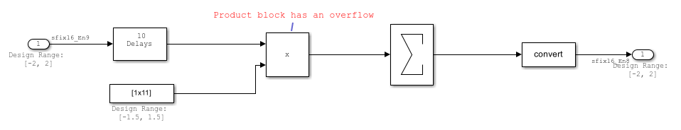
Known design minimum and maximum values are specified explicitly on blocks in the model, including on the inputs and outputs of the Embedded Efficient Filter subsystem.
Open the Fixed-Point Tool. On the Simulink® Apps tab, under Code Generation, click the app icon.
To start the range collection workflow, select Range Collection.
Select the subsystem that you want to analyze. Under System Under Design (SUD), select the Embedded Efficient Filter subsystem.
Choose the range collection method to use. Under Range Collection Mode, select Simulation with derived ranges. During range collection, the tool will combine ranges from simulation minimum and maximum values, design minimum and maximum values specified explicitly on blocks in the model, and derived minimum and maximum values that are computed through a static analysis that derived ranges for objects in the model.
Specify Simulation Inputs. For this example, use the default model inputs for simulation.
Specify signal tolerances for logged signals. Set the Absolute Tolerance and Relative Tolerance of the output_signal:1 to 0.01.

Next, expand the Collect Ranges button arrow to configure the settings to use for range collection. Select Double precision to temporarily override data types in the model with doubles during the baseline range collection run. Click Collect Ranges.

The results of the range collection run are stored in BaselineRun. The Results spreadsheet displays a summary of the statistics collected during the range collection, including the currently specified data types on the model (SpecifiedDT), simulation minimum, and simulation maximum values. The compiled data type (CompiledDT) column displays double for all objects in the Embedded Efficient Filter subsystem, indicating that data type override was applied during the range collection simulation.

You can click on any result to view additional details in the Result Details pane. The Visualization of Simulation Data pane displays a summary of histograms of the bits used by each object in your model.
You can customize the information displayed in the Results spreadsheet, or use the Explore tab to sort and filter these results based on additional criteria. For more information, see Control Views in the Fixed-Point Tool.
Next, simulate the model using the fixed-point data types currently specified on the model. Expand the Settings button arrow and select Specified data types, then click Simulate with Embedded Types.
The Fixed-Point Tool stores the results of the simulation in EmbeddedRun.

The icon next to EmbeddedRun displays a fail status, indicating that one or more signals do not meet the specified tolerances. The results for the Product block indicate that there is an issue with this result. The Result Details pane shows that the block overflowed 1670 times, indicating a poor choice of word length.
To compare the ideal results stored in BaselineRun with the fixed-point results, select EmbeddedRun from the Run to compare in SDI drop down menu. Then click Compare Results to open the Simulation Data Inspector. In the Simulation Data Inspector, select output_signal as the signal to compare.

Related Examples
Parameters
Limitations
Some blocks do not support fixed-point data types and can result in an error during fixed-point conversion. See Blocks That Do Not Support Fixed-Point Data Types.
Some modeling constructs may cause data type propagation issues. See Models That Might Cause Data Type Propagation Errors.
If your model contains a MATLAB Function block, use only supported modeling constructs for successful conversion. See Best Practices for Working with the MATLAB Function Block in Automated Fixed-Point Conversion Workflows.
If your system contains a model reference hierarchy using the Model block, see Considerations for Working with Model References in Fixed-Point Conversion Workflows.
The tool does not convert non-writable or read-only blocks or subsystems, including linked library blocks. Read-only constructs are surrounded by Data Type Conversion blocks during the Unsupported Constructs preparation check.
Tips
For best practices and recommendations, see Best Practices for Fixed-Point Conversion Workflow.
To customize views in the Fixed-Point Tool, see Control Views in the Fixed-Point Tool.
For help troubleshooting the optimization workflow, see Data Type Optimization Not Successful.