Vehicle Path Tracking Using Pure Pursuit Controller
From the series: Improving Your Racecar Development
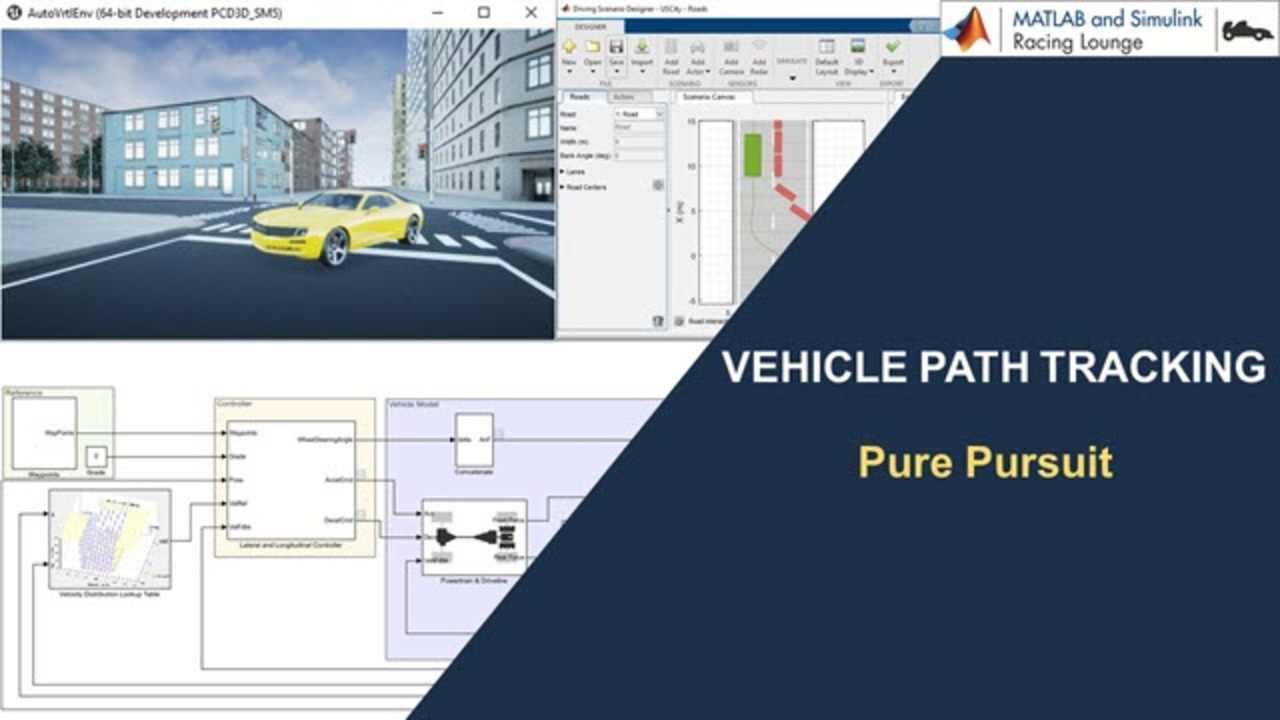
Learn how to implement a pure pursuit controller on an autonomous vehicle to track a planned path. Veer introduces the basics of a pure pursuit controller and shows the steps to model a vehicle with using the Automated Driving Toolbox™, Vehicle Dynamics Blockset™, Robotics System Toolbox™ and Navigation Toolbox™. He implements the longitudinal and lateral controllers to track the path with high velocity and extracts the waypoints to drive the vehicle through a US city scene. He also demonstrates the model to visualize the vehicle motion in a 3D environment and bird’s-eye view.
You can find the example models used in this video on MATLAB Central File Exchange.
For more information, you can access the following resources:
Published: 20 Jul 2020
Hello and welcome to the MATLAB and Simulink Racing Lounge. In this video, we'll show how to implement a Pure pursuit controller on a vehicle for path tracking. We'll see how you can build a vehicle path tracking model in Simulink and visualize the motion in various environments. We'll go through some other basics of the Pure Pursuit, controller, then we'll have a section for an implementation using Simulink, and finally, we'll go to the key takeaways.
So now, let's get started. The Pure Pursuit controller is a path tracking algorithm where we place a waypoint, a reference point, and a path at a fixed distance ahead, which is also called look ahead distance of the vehicle, and calculate the steering command to intersect at this point. As the vehicle turns towards the reference spot, the point continues to move forward, reducing the steering angle, and slowly bringing the vehicle on the path.
The look ahead distance is the main tuning property of the controller. The figure shows the effect of look ahead distance on a vehicle in motion. For a smaller look ahead distance, the path is oscillatory and accurate. And for a larger look at a distance, the part it's less oscillatory, but the tracking is poor.
Further, this is a formula for calculating the wheel steering angle where L is the bicycle length and ld is the look ahead distance, an alpha is a target direction angle, and the same can be also seen in the figure. Moving ahead, here are the steps involved in implementing the Pure Pursuit controller using Simulink. As a first step, we generate the waypoints or reference points, then we build a model in Simulink, and finally, we visualize the vehicle motion in various environments such as 2D, 3D, and bird's-eye scope.
So now let's switch to MATLAB and check out these steps in detail. To generate the waypoints, we use a Driving Scenario Designer, where we have defined the route and added the waypoints for the vehicle to move at a constant velocity. For more information on various other capabilities of Driving Scenario Designer, please check out the links provided in the description.
Further, the scene is set as a .mat file that contains data for the reference spot. To extract the data, we have created a script where we can see these are the commands to define the reference spot. Further, the script also contains data for defining the reference submission time, vehicle parameters, and the controller's initial tuning parameters.
Once we have these reference points and initial parameters set, let's check out how we have built the model in Simulink. To the Simulink blank canvas, we bring in a "Vehicle Body 3DOF Dual Track" block from the Vehicle Dynamics Blockset, and then define certain initial values to implement a vehicle body model. Next, we define the reference spot in x and y directions. To implement a Pure Pursuit controller, we use a Pure Pursuit block from the robotic system toolbox, where we define the look ahead distance and check the target direction to output the target angle.
As the input of waypoint board accepts the signal in the form of the n-by-2 array, we convert a different signal using a concatenate block. Next, we extract the vehicle current pose from the vehicle 3DOF Dual Track block using a Bus Selector, and use a MUX signal to convert these into a vector accepted by the pose input board. Further, we use some basic blocks to formulate the wheel steering angle, referring to the formula shown earlier.
Here, alpha is the target direction angle that is provided by the Pure Pursuit block, and then connect the former wheel steering angle to the vehicle block using a concatenate block to complete the model. Please note that, as an alternative, we can also connect the output linear velocity port of the Pure Pursuit block to move the vehicle with a constant velocity. However, since in later models we'll be adding some more dynamics and a longitudinal controller, we will stick with a constant block to define the velocity. To learn more about implementing Pure Pursuit controller for a differential drive report, just check the links in the description.
In short, this was a procedure to show how you can easily connect blocks to build a model in Simulink. Now, we have restructured the same model where we have included the wheel steering angle formulation in a subsystem and added a mask to define the bicycle length and look ahead distance. Further, we have added a 2D visualization block and cleaned the model using some subsystems.
So let's run the model and get the results. As we can see, with the correct selection of the look ahead distance, the vehicle is successfully able to track the reference spot. We can also visualize the steering angle, which is very well within the limits of passenger vehicles.
Now, let's check out the effect of changing the look ahead distance. As we decrease the look ahead distance, the vehicle does track the path, but the path is oscillatory, whereas, increasing the look ahead distance removes the oscillatory motion, but at the cost of poorer tracking. Hence, the look ahead distance should be selected properly to keep a balance between the tracking and the stability of the vehicle.
Now, let's increase the velocity and see the effect of the vehicle in motion. So we increase the velocity to 15 meters per second and we see lower efficient tracking at the turns. Now one way to improve the tracking could be to reduce the velocity at the turns and add a longitudinal controller to track the difference velocity.
So let's check out that model. Hence, if we move ahead to our next model where we add more dynamics and a longitudinal controller, compared to the last model, in this model, we have added a simplified block for powertrain and drivetrain. For this, we have referred to the scene interrogation difference application. To know more about this, please go to the video description, where we have provided the link.
In the controller subsystem, we have added a longitudinal driver to track the reference velocity. The block stakes in the reference velocity, longitudinal vehicle velocity, and create as input signals and outputs acceleration and deceleration command based on the type of controller and selected dual control parameters. Next, we have divided the velocity into different regions. For example, low velocity at turns and a built-in lookup table, which looks like this. And this block calculates the velocity in that region based on x and y coordinates. Apart from that, there is no major change in the model.
Now let's run the simulation. And as we can see, that now we have much better tracking at the turns because of the longitudinal controller. Having seen the model with the longitudinal and lateral controller at high velocity, let's send the vehicle to a city scene. So far that, we use the driving scenario designer to generate the reference points.
However, rather than creating the scene from scratch, we use prebuilt scenarios, where we can see various prebuilt scenes. Here, we select a US city block scene. And when we select this, the scene can be visualized in the scenario canvas with various actors.
So to this scene, we have already added the vehicle and defined the way points to move the vehicle without colliding with any of the obstacles. Now, we have built a new model referring to the previous models we are following at the modifications. The waypoint subsystem contains the data for the US city scene.
Then, we have changed the lookup table for the velocity where we have divided the velocity into five regions. We start with 12 meters per second, and during turns, the velocity reduces to 5 meters per second. And similarly, we have different velocity in different regions. Finally, we have added some additional blocks for visualization.
The simulation 3D vehicle with ground following block implements a vehicle in a 3D visualization environment, where we need to define the vehicle parameters. Further, simulation 3D scene configuration block configures a 3D simulation environment, where we can select the scene source and scene name. For this model, as we have extracted the reference points from the US city scene in the driving scenario designer, we will select the same scene to visualize the vehicle motion in the 3D environment.
Having configured the 3D scene, now let's run the simulation. As you can see, the vehicle is successfully tracking the reference spot without colliding with any of the obstacles. Now, to visualize the path in a bird's-eye scope, we have added a subsystem where the MATLAB function packs the Ego information into a single egoActor Bus, and a driving scenario reader block reads the scenario file.
To activate the bird's-eye scope, click on the tab here, which shows a blank scope canvas with no signals. To see the signals, click find signals. The scope updates a block diagram and automatically finds the signals in the model. So once again, when we run the simulation, we can visualize the vehicle motion in bird's-eye scope, where the vehicle is successfully tracking the reference spot without colliding with any of the actors.
So this was our final model where we saw how we can drive the vehicle through a prebuilt scene using a Pure Pursuit and along a longitudinal controller. In case you are interested to learn about other controllers, such as Stanley and MBC, please check out the links in the description.
Now let's move ahead and check out the key takeaways. As we saw, the look ahead distance is the main tuning property of the Pure Pursuit controller. That is, the way we tune the look ahead distance will effect the vehicle in motion. Then at higher velocities and varying curvatures, combining lateral and longitudinal controllers give better part tracking results. And finally, MATLAB and Simulink provide various algorithms and tools for generating waypoints, building vehicle and controller models, and visualizing the vehicle motion in various environments.
And as usual, these are the Racing Lounge Resources. If you have any queries, reach out to racinglounge@mathworks.com, and we would also encourage you to join our Facebook group to check out the latest updates and also check out our student tutorials and Racing Lounge blog.


